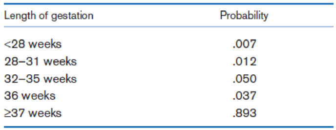
Obstetrics The following data are derived from the Monthly Vital Statistics Report (October 1999) issued by the National Center for Health Statistics [10]. These data are pertinent to livebirths only. Suppose that infants are classified as low birthweight if they have a birthweight <2500 g and as normal birthweight if they have a birthweight ≥2500 g. Suppose that infants are also classified by length of gestation in the following five categories: <28 weeks, 28–31 weeks, 32–35 weeks, 36 weeks, and ≥37 weeks. Assume the probabilities of the different periods of gestation are as given in Table 3.8. Also assume that the probability of low birthweight is .949 given a gestation of <28 weeks, .702 given a gestation of 28–31 weeks, .434 given a gestation of 32–35 weeks, .201 given a gestation of 36 weeks, and .029 given a gestation of ≥37 weeks. Table 3.8 Distribution of length of gestation What is the probability of having a length of gestation ≤36 weeks given that an infant is low birthweight?
Obstetrics The following data are derived from the Monthly Vital Statistics Report (October 1999) issued by the National Center for Health Statistics [10]. These data are pertinent to livebirths only. Suppose that infants are classified as low birthweight if they have a birthweight <2500 g and as normal birthweight if they have a birthweight ≥2500 g. Suppose that infants are also classified by length of gestation in the following five categories: <28 weeks, 28–31 weeks, 32–35 weeks, 36 weeks, and ≥37 weeks. Assume the probabilities of the different periods of gestation are as given in Table 3.8. Also assume that the probability of low birthweight is .949 given a gestation of <28 weeks, .702 given a gestation of 28–31 weeks, .434 given a gestation of 32–35 weeks, .201 given a gestation of 36 weeks, and .029 given a gestation of ≥37 weeks. Table 3.8 Distribution of length of gestation What is the probability of having a length of gestation ≤36 weeks given that an infant is low birthweight?
The following data are derived from the Monthly Vital Statistics Report (October 1999) issued by the National Center for Health Statistics [10]. These data are pertinent to livebirths only.
Suppose that infants are classified as low birthweight if they have a birthweight <2500 g and as normal birthweight if they have a birthweight ≥2500 g. Suppose that infants are also classified by length of gestation in the following five categories: <28 weeks, 28–31 weeks, 32–35 weeks, 36 weeks, and ≥37 weeks. Assume the probabilities of the different periods of gestation are as given in Table 3.8.
Also assume that the probability of low birthweight is .949 given a gestation of <28 weeks, .702 given a gestation of 28–31 weeks, .434 given a gestation of 32–35 weeks, .201 given a gestation of 36 weeks, and .029 given a gestation of ≥37 weeks.
Table 3.8 Distribution of length of gestation
What is the probability of having a length of gestation ≤36 weeks given that an infant is low birthweight?
Harvard University
California Institute of Technology
Massachusetts Institute of Technology
Stanford University
Princeton University
University of Cambridge
University of Oxford
University of California, Berkeley
Imperial College London
Yale University
University of California, Los Angeles
University of Chicago
Johns Hopkins University
Cornell University
ETH Zurich
University of Michigan
University of Toronto
Columbia University
University of Pennsylvania
Carnegie Mellon University
University of Hong Kong
University College London
University of Washington
Duke University
Northwestern University
University of Tokyo
Georgia Institute of Technology
Pohang University of Science and Technology
University of California, Santa Barbara
University of British Columbia
University of North Carolina at Chapel Hill
University of California, San Diego
University of Illinois at Urbana-Champaign
National University of Singapore
McGill…
Name
Harvard University
California Institute of Technology
Massachusetts Institute of Technology
Stanford University
Princeton University
University of Cambridge
University of Oxford
University of California, Berkeley
Imperial College London
Yale University
University of California, Los Angeles
University of Chicago
Johns Hopkins University
Cornell University
ETH Zurich
University of Michigan
University of Toronto
Columbia University
University of Pennsylvania
Carnegie Mellon University
University of Hong Kong
University College London
University of Washington
Duke University
Northwestern University
University of Tokyo
Georgia Institute of Technology
Pohang University of Science and Technology
University of California, Santa Barbara
University of British Columbia
University of North Carolina at Chapel Hill
University of California, San Diego
University of Illinois at Urbana-Champaign
National University of Singapore…
A company found that the daily sales revenue of its flagship product follows a normal distribution with a mean of $4500 and a standard deviation of $450. The company defines a "high-sales day" that is, any day with sales exceeding $4800. please provide a step by step on how to get the answers in excel
Q: What percentage of days can the company expect to have "high-sales days" or sales greater than $4800?
Q: What is the sales revenue threshold for the bottom 10% of days? (please note that 10% refers to the probability/area under bell curve towards the lower tail of bell curve)
Provide answers in the yellow cells
Need a deep-dive on the concept behind this application? Look no further. Learn more about this topic, statistics and related others by exploring similar questions and additional content below.
Continuous Probability Distributions - Basic Introduction; Author: The Organic Chemistry Tutor;https://www.youtube.com/watch?v=QxqxdQ_g2uw;License: Standard YouTube License, CC-BY
Probability Density Function (p.d.f.) Finding k (Part 1) | ExamSolutions; Author: ExamSolutions;https://www.youtube.com/watch?v=RsuS2ehsTDM;License: Standard YouTube License, CC-BY
Find the value of k so that the Function is a Probability Density Function; Author: The Math Sorcerer;https://www.youtube.com/watch?v=QqoCZWrVnbA;License: Standard Youtube License


 Glencoe Algebra 1, Student Edition, 9780079039897...AlgebraISBN:9780079039897Author:CarterPublisher:McGraw Hill
 College Algebra (MindTap Course List)AlgebraISBN:9781305652231Author:R. David Gustafson, Jeff HughesPublisher:Cengage Learning
 Holt Mcdougal Larson Pre-algebra: Student Edition...AlgebraISBN:9780547587776Author:HOLT MCDOUGALPublisher:HOLT MCDOUGAL
 Big Ideas Math A Bridge To Success Algebra 1: Stu...AlgebraISBN:9781680331141Author:HOUGHTON MIFFLIN HARCOURTPublisher:Houghton Mifflin Harcourt
 Functions and Change: A Modeling Approach to Coll...AlgebraISBN:9781337111348Author:Bruce Crauder, Benny Evans, Alan NoellPublisher:Cengage Learning
 Linear Algebra: A Modern IntroductionAlgebraISBN:9781285463247Author:David PoolePublisher:Cengage Learning