
Videos
The paper “Lessons from Pacemaker Implantations” (Journal of the American Medical Association [1965]: 231–232) gave the results of a study that followed 89 heart patients who had received electronic pacemakers. The time (in months) to the first electrical malfunction of the pacemaker was recorded:
![Chapter 3, Problem 12CRE, The paper Lessons from Pacemaker Implantations (Journal of the American Medical Association [1965]:](https://content.bartleby.com/tbms-images/9781337793612/Chapter-3/images/93612-3-12cre-question-digital_image_001.png)
- a. Summarize these data in the form of a frequency distribution, using class intervals of 0 to <6, 6 to <12, and so on.
- b. Calculate the relative frequencies and cumulative relative frequencies for each class interval of the frequency distribution of Part (a).
- c. Show how the relative frequency for the class interval 12 to <18 could be obtained from the cumulative relative frequencies.
- d. Use the cumulative relative frequencies to give approximate answers to the following:
- i. What proportion of those who participated in the study had pacemakers that did not malfunction within the first year?
- ii. If the pacemaker must be replaced as soon as the first electrical malfunction occurs, approximately what proportion required replacement between 1 and 2 years after implantation?
- e. Construct a cumulative relative frequency plot, and use it to answer the following questions.
- i. What is the approximate time at which 50% of the pacemakers had failed?
- ii. What is the approximate time at which only 10% of the pacemakers initially implanted were still
functioning ?
a.
Construct the frequency distribution for the given data.
Answer to Problem 12CRE
The frequency distribution is given below.
| Class interval | Frequency |
| 0-<6 | 2 |
| 6-<12 | 10 |
| 12-<18 | 21 |
| 18-<24 | 28 |
| 24-<30 | 22 |
| 30-<36 | 6 |
Explanation of Solution
Calculation:
The data represents the time to the first electrical malfunction of the pacemaker for 89 heart patients.
Software procedure:
Frequency distribution:
The number of values lying in the particular interval or the number of times each value repeats is the frequency of that particular class interval or event.
The frequencies are calculated by using the tally mark. Here, the number of times each activity repeats is the frequency of that particular physical activity.
Here, the number of values time under the specified interval is the frequency of that particular class interval of time.
Here, the number of values in between the class interval 0-<6 is 2.
Therefore, the frequency of the class interval 0-<6 is 2.
Similarly, the frequencies of all the remaining class intervals are as follows:
| Class interval | Tally | Frequency |
| 0-<6 | 2 | |
| 6-<12 | 10 | |
| 12-<18 | 21 | |
| 18-<24 | 28 | |
| 24-<30 | 22 | |
| 30-<36 | 6 | |
| Total | 89 |
b.
Construct the relative frequency distribution for the given data.
Construct the cumulative relative frequency distribution for the given data.
Answer to Problem 12CRE
The relative frequency distribution and cumulative relative frequency distribution are given below.
| Class interval | Relative frequency | Cumulative relative frequency |
| 0-<6 | 0.02247 | 0.02247 |
| 6-<12 | 0.11236 | 0.13483 |
| 12-<18 | 0.23596 | 0.37079 |
| 18-<24 | 0.31461 | 0.6854 |
| 24-<30 | 0.24719 | 0.39259 |
| 30-<36 | 0.06742 | 1 |
Explanation of Solution
Calculation:
The general formula to obtain the relative frequency is given below:
Substitute the frequency of the class interval 0-<6 as “2” and the total frequency as “89” in relative frequency.
Similarly, relative frequencies for the remaining class intervals are obtained below:
| Class interval | Frequency | Relative frequency |
| 0-<6 | 2 | |
| 6-<12 | 10 | |
| 12-<18 | 21 | |
| 18-<24 | 28 | |
| 24-<30 | 22 | |
| 30-<36 | 6 |
Cumulative relative frequency:
Cumulative relative frequency is the sum of relative frequencies of all the previous events which are arranged in an order from smallest to largest value.
The general formula to obtain cumulative frequency using frequency distribution is,
From the relative frequencies, the cumulative relative frequencies are obtained as follows:
| Class interval | Relative frequency | Cumulative relative frequency |
| 0-<6 | 0.02247 | |
| 6-<12 | 0.11236 | |
| 12-<18 | 0.23596 | |
| 18-<24 | 0.31461 | |
| 24-<30 | 0.24719 | |
| 30-<36 | 0.06742 |
c.
Obtain the relative frequency for the class interval 12-18 using the cumulative frequency distribution.
Answer to Problem 12CRE
The relative frequency for the class interval 12-18 using the cumulative frequency distribution is 0.23596.
Explanation of Solution
Calculation:
The general formula to obtain cumulative frequency using frequency distribution is given below:
Relative frequency of a present event is obtained using the formula given below:
From the cumulative relative frequency distribution, relative frequency distribution is obtained as given below:
Thus, the relative frequency for the class interval 12-18 using the cumulative frequency distribution is 0.23596.
d.
(i). Find the approximate proportion of heart patients who had pacemakers that did not malfunction within the first year.
(ii) Find the approximate proportion of heart patients who required replacement between 1 and 2 years after implantation.
Answer to Problem 12CRE
(i) The approximate proportion of heart patients who had pacemakers that did not malfunction within the first year is 0.86517.
(ii) The approximate proportion of heart patients who required replacement between 1 and 2 years after implantation is 0.55057.
Explanation of Solution
Calculation:
The general formula for the relative frequency or proportion is,
(i). Approximate proportion of heart patients who had pacemakers that did not malfunction within the first year:
The Objective is to find the cumulative relative frequency of heart patients who had pacemakers that did not malfunction within the first year.
The cumulative relative frequency of heart patients who had pacemakers that malfunction within the first year is 0.13483.
That is, the proportion of heart patients who had pacemakers that malfunction within the first year is 0.13483.
Hence, the cumulative relative frequency of heart patients who had pacemakers that did not malfunction within the first year is obtained as given below:
Thus, the approximate proportion of heart patients who had pacemakers that did not malfunction within the first year is 0.86517.
(ii). Approximate proportion of heart patients who required replacement between 1 and 2 years after implantation:
The Objective is to find the relative frequency of heart patients required replacement between 1 and 2 years after implantation.
The relative frequency of heart patients required replacement between 1 and 2 years after implantation is obtained as given below:
Thus, the approximate proportion of heart patients who required replacement between 1 and 2 years after implantation is 0.55057.
e.
Plot the cumulative frequency distribution for the given data.
(i) Find the approximate time at which 50% of the pacemakers had failed.
(ii) Find the approximate time at which only 10% of the initially implanted pacemakers are functioning.
Answer to Problem 12CRE
Cumulative distribution plot is given below:
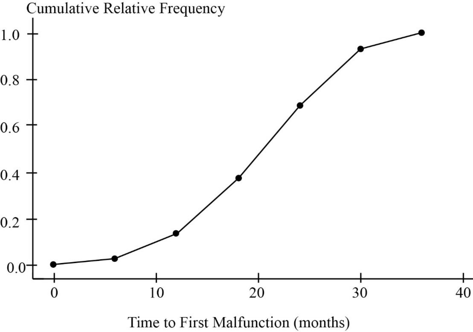
(i) The time at which 50% of the pacemakers had failed will be in between 18-<24 months.
(ii) The approximate time at which only 10% of the initially implanted pacemakers are functioning will be in between 24-<30 months.
Explanation of Solution
Calculation:
The cumulative relative frequency histogram is plotted for the given data.
Procedure to plot cumulative distribution plot:
Step by step procedure to draw the cumulative distribution plot is given below.
- Draw a horizontal axis and a vertical axis.
- The horizontal axis represents the cumulative frequencies.
- The vertical axis represents the “Time to first malfunction in months”.
- Plot each of the 6 cumulative frequencies corresponding to the time to first malfunction in months.
- Connect all the 6 plotted points of cumulative frequencies with a line.
The general formula for the relative frequency or proportion is,
(i). Approximate time at which 50% of the pacemakers had failed:
The Objective is to find the time at which 50% of the pacemakers had failed.
From the cumulative relative frequency distribution, 0.6854 corresponds to the interval 18-<24 months.
The cumulative relative frequency of 0.5 is less than the cumulative relative frequency of 0.6854.
Thus, the time at which 50% of the pacemakers had failed will be in between 18-<24 months.
(ii). Approximate time at which only 10% of the initially implanted pacemakers are functioning:
The Objective is to find the time only 10% of the initially implanted pacemakers are functioning.
In other words it can be said that, the time at which 90% of the pacemakers had failed.
From the cumulative relative frequency distribution, 0.93259 corresponds to the interval 24-<30 months.
The cumulative relative frequency of 0.9 is less than the cumulative relative frequency of 0.93259.
Thus, the time at which only 10% of the initially implanted pacemakers are functioning will be in between 24-<30 months.
Want to see more full solutions like this?
Chapter 3 Solutions
Introduction to Statistics and Data Analysis
Additional Math Textbook Solutions
Pathways To Math Literacy (looseleaf)
College Algebra (Collegiate Math)
Elementary and Intermediate Algebra: Concepts and Applications (7th Edition)
Precalculus
Elementary Statistics ( 3rd International Edition ) Isbn:9781260092561
APPLIED STAT.IN BUS.+ECONOMICS


- « CENGAGE MINDTAP Quiz: Chapter 38 Assignment: Quiz: Chapter 38 ips Questions ra1kw08h_ch38.15m 13. 14. 15. O Which sentence has modifiers in the correct place? O a. When called, she for a medical emergency responds quickly. b. Without giving away too much of the plot, Helena described the heroine's actions in the film. O c. Nearly the snakebite victim died before the proper antitoxin was injected. . O O 16 16. O 17. 18. O 19. O 20 20. 21 21. 22. 22 DS 23. 23 24. 25. O O Oarrow_forwardQuestions ra1kw08h_ch36.14m 12. 13. 14. 15. 16. Ӧ 17. 18. 19. OS 20. Two separate sentences need Oa. two separate subjects. Ob. two dependent clauses. c. one shared subject.arrow_forwardCustomers experiencing technical difficulty with their Internet cable service may call an 800 number for technical support. It takes the technician between 30 seconds and 11 minutes to resolve the problem. The distribution of this support time follows the uniform distribution. Required: a. What are the values for a and b in minutes? Note: Do not round your intermediate calculations. Round your answers to 1 decimal place. b-1. What is the mean time to resolve the problem? b-2. What is the standard deviation of the time? c. What percent of the problems take more than 5 minutes to resolve? d. Suppose we wish to find the middle 50% of the problem-solving times. What are the end points of these two times?arrow_forward
- Exercise 6-6 (Algo) (LO6-3) The director of admissions at Kinzua University in Nova Scotia estimated the distribution of student admissions for the fall semester on the basis of past experience. Admissions Probability 1,100 0.5 1,400 0.4 1,300 0.1 Click here for the Excel Data File Required: What is the expected number of admissions for the fall semester? Compute the variance and the standard deviation of the number of admissions. Note: Round your standard deviation to 2 decimal places.arrow_forward1. Find the mean of the x-values (x-bar) and the mean of the y-values (y-bar) and write/label each here: 2. Label the second row in the table using proper notation; then, complete the table. In the fifth and sixth columns, show the 'products' of what you're multiplying, as well as the answers. X y x minus x-bar y minus y-bar (x minus x-bar)(y minus y-bar) (x minus x-bar)^2 xy 16 20 34 4-2 5 2 3. Write the sums that represents Sxx and Sxy in the table, at the bottom of their respective columns. 4. Find the slope of the Regression line: bi = (simplify your answer) 5. Find the y-intercept of the Regression line, and then write the equation of the Regression line. Show your work. Then, BOX your final answer. Express your line as "y-hat equals...arrow_forwardApply STATA commands & submit the output for each question only when indicated below i. Generate the log of birthweight and family income of children. Name these new variables Ibwght & Ifaminc. Include the output of this code. ii. Apply the command sum with the detail option to the variable faminc. Note: you should find the 25th percentile value, the 50th percentile and the 75th percentile value of faminc from the output - you will need it to answer the next question Include the output of this code. iii. iv. Use the output from part ii of this question to Generate a variable called "high_faminc" that takes a value 1 if faminc is less than or equal to the 25th percentile, it takes the value 2 if faminc is greater than 25th percentile but less than or equal to the 50th percentile, it takes the value 3 if faminc is greater than 50th percentile but less than or equal to the 75th percentile, it takes the value 4 if faminc is greater than the 75th percentile. Include the outcome of this code…arrow_forward
- solve this on paperarrow_forwardApply STATA commands & submit the output for each question only when indicated below i. Apply the command egen to create a variable called "wyd" which is the rowtotal function on variables bwght & faminc. ii. Apply the list command for the first 10 observations to show that the code in part i worked. Include the outcome of this code iii. Apply the egen command to create a new variable called "bwghtsum" using the sum function on variable bwght by the variable high_faminc (Note: need to apply the bysort' statement) iv. Apply the "by high_faminc" statement to find the V. descriptive statistics of bwght and bwghtsum Include the output of this code. Why is there a difference between the standard deviations of bwght and bwghtsum from part iv of this question?arrow_forwardAccording to a health information website, the distribution of adults’ diastolic blood pressure (in millimeters of mercury, mmHg) can be modeled by a normal distribution with mean 70 mmHg and standard deviation 20 mmHg. b. Above what diastolic pressure would classify someone in the highest 1% of blood pressures? Show all calculations used.arrow_forward
- Write STATA codes which will generate the outcomes in the questions & submit the output for each question only when indicated below i. ii. iii. iv. V. Write a code which will allow STATA to go to your favorite folder to access your files. Load the birthweight1.dta dataset from your favorite folder and save it under a different filename to protect data integrity. Call the new dataset babywt.dta (make sure to use the replace option). Verify that it contains 2,998 observations and 8 variables. Include the output of this code. Are there missing observations for variable(s) for the variables called bwght, faminc, cigs? How would you know? (You may use more than one code to show your answer(s)) Include the output of your code (s). Write the definitions of these variables: bwght, faminc, male, white, motheduc,cigs; which of these variables are categorical? [Hint: use the labels of the variables & the browse command] Who is this dataset about? Who can use this dataset to answer what kind of…arrow_forwardApply STATA commands & submit the output for each question only when indicated below İ. ii. iii. iv. V. Apply the command summarize on variables bwght and faminc. What is the average birthweight of babies and family income of the respondents? Include the output of this code. Apply the tab command on the variable called male. How many of the babies and what share of babies are male? Include the output of this code. Find the summary statistics (i.e. use the sum command) of the variables bwght and faminc if the babies are white. Include the output of this code. Find the summary statistics (i.e. use the sum command) of the variables bwght and faminc if the babies are male but not white. Include the output of this code. Using your answers to previous subparts of this question: What is the difference between the average birthweight of a baby who is male and a baby who is male but not white? What can you say anything about the difference in family income of the babies that are male and male…arrow_forwardA public health researcher is studying the impacts of nudge marketing techniques on shoppers vegetablesarrow_forward
 Glencoe Algebra 1, Student Edition, 9780079039897...AlgebraISBN:9780079039897Author:CarterPublisher:McGraw Hill
 Functions and Change: A Modeling Approach to Coll...AlgebraISBN:9781337111348Author:Bruce Crauder, Benny Evans, Alan NoellPublisher:Cengage Learning
 Holt Mcdougal Larson Pre-algebra: Student Edition...AlgebraISBN:9780547587776Author:HOLT MCDOUGALPublisher:HOLT MCDOUGAL