
Videos
a.
Construct the frequency distribution with approximately 5classes.
a.
Answer to Problem 31E
The frequency distribution is,
| Number of Words | Frequency |
| 0-1,999 | 26 |
| 2,000-3,999 | 25 |
| 4,000-5,999 | 5 |
| 6,000-7,999 | 0 |
| 8,000-9,999 | 1 |
| Total | 57 |
Explanation of Solution
Calculation:
The given information is that a table representing the number of words spoken in each of these addresses.
Frequency:
The frequencies are calculated by using the tally mark and the
- Based on the given information, the class intervals are 0-1,999, 2,000-3,999, 4,000-5,999, 6,000-7,999, 8,000-9,999.
- Make a tally mark for each value in the corresponding number of words spoken and continue for all values in the data.
- The number of tally marks in each class represents the frequency, f of that class.
Similarly, the frequency of remaining classes for the number of words spoken is given below:
| Number of Words | Tally | Frequency |
| 0-1,999 | 26 | |
| 2,000-3,999 | 25 | |
| 4,000-5,999 | 5 | |
| 6,000-7,999 | 0 | |
| 8,000-9,999 | 1 | |
| Total | 57 |
b.
Construct the frequency histogram based on the frequency distribution.
b.
Answer to Problem 31E
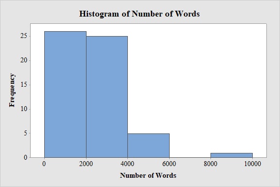
Output obtained from MINITAB software for the number of words spoken is:
Explanation of Solution
Calculation:
Frequency Histogram:
Software procedure:
- Step by step procedure to draw the relative frequency histogram for number of words spoken using MINITAB software.
- Choose Graph > Histogram.
- Choose Simple.
- Click OK.
- In Graph variables, enter the column of Number of Words.
- In Scale, Choose Y-scale Type as Frequency.
- Click OK.
- Select Edit Scale, Enter 0, 2,000, 4,000, 6,000, 8,000, 10,000 in Positions of ticks.
- In Binning, Under Interval Type select Cutpoint and under Interval Definition select Number of intervals as 5 and Cutpoint positions as 0, 2,000, 4,000, 6,000, 8,000, 10,000.
- In Labels, Enter 0, 2,000, 4,000, 6,000, 8,000, 10,000 in Specified.
- Click OK.
Observation:
From the bar graph, it can be seen that maximum number of words spoken are in the interval 0-2,000.
c.
Construct a relative frequency distribution for the data.
c.
Answer to Problem 31E
The relative frequency distribution for the data is:
| Number of Words | Relative frequency |
| 0-1,999 | 0.456 |
| 2,000-3,999 | 0.439 |
| 4,000-5,999 | 0.088 |
| 6,000-7,999 | 0.000 |
| 8,000-9,999 | 0.018 |
Explanation of Solution
Calculation:
Relative frequency:
The general formula for the relative frequency is,
Therefore,
Similarly, the relative frequencies for the remaining number of words spoken are obtained below:
| Number of Words | Frequency | Relative frequency |
| 0-1,999 | 26 | |
| 2,000-3,999 | 25 | |
| 4,000-5,999 | 5 | |
| 6,000-7,999 | 0 | |
| 8,000-9,999 | 1 |
d.
Construct the relative frequency histogram based on the frequency distribution.
d.
Answer to Problem 31E
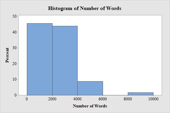
Output obtained from MINITAB software for the number of words spoken is:
Explanation of Solution
Calculation:
Relative Frequency Histogram:
Software procedure:
- Step by step procedure to draw the relative frequency histogram for the number of words spoken using MINITAB software.
- Choose Graph > Histogram.
- Choose Simple.
- Click OK.
- In Graph variables, enter the column of Number of Words.
- In Scale, Choose Y-scale Type as Percent.
- Click OK.
- Select Edit Scale, Enter 0, 2,000, 4,000, 6,000, 8,000, 10,000 in Positions of ticks.
- In Binning, Under Interval Type select Cutpoint and under Interval Definition select Number of intervals as 5 and Cutpoint positions as 0, 2,000, 4,000, 6,000, 8,000, 10,000.
- In Labels, Enter 0, 2,000, 4,000, 6,000, 8,000, 10,000 in Specified.
- Click OK.
Observation:
From the bar graph, it can be seen that maximum number of words spoken is in the interval 0-2,000.
e.
Check whether the histograms are skewed to the left, skewed to the right or approximately symmetric.
e.
Answer to Problem 31E
The histogram is skewed to the right.
Explanation of Solution
From the given histogram, the right hand tail is larger than the left hand tail from the maximum frequency value. Hence, the shape of the distribution is right skewed.
f.
Construct the frequency distribution with approximately 9classes.
f.
Answer to Problem 31E
The frequency distribution is,
| Number of Words | Frequency |
| 0-999 | 4 |
| 1,000-1,999 | 22 |
| 2,000-2,999 | 18 |
| 3,000-3,999 | 7 |
| 4,000-4,999 | 4 |
| 5,000-5,999 | 1 |
| 6,000-6,999 | 0 |
| 7,000-7,999 | 0 |
| 8,000-8,999 | 1 |
| Total | 57 |
Explanation of Solution
Calculation:
Frequency:
The frequencies are calculated by using the tally mark and the range of the data is from 0 to 8,999.
- Based on the given information, the class intervals are 0-999, 1,000-1,999, 2,000-2,999, 3,000-3,999, 4,000-4,999, 5,000-5,999, 6,000-6,999, 7,000-7,999, 8,000-8,999.
- Make a tally mark for each value in the corresponding number of words spoken and continue for all values in the data.
- The number of tally marks in each class represents the frequency, f of that class.
Similarly, the frequency of remaining classes for the number of words spoken is given below:
| Number of Words | Tally | Frequency |
| 0-999 | 4 | |
| 1,000-1,999 | 22 | |
| 2,000-2,999 | 18 | |
| 3,000-3,999 | 7 | |
| 4,000-4,999 | 4 | |
| 5,000-5,999 | 1 | |
| 6,000-6,999 | 0 | |
| 7,000-7,999 | 0 | |
| 8,000-8,999 | 1 | |
| Total | 57 |
g.
Repeat parts (b) to (d), using the frequency distribution constructed in part (f).
g.
Answer to Problem 31E
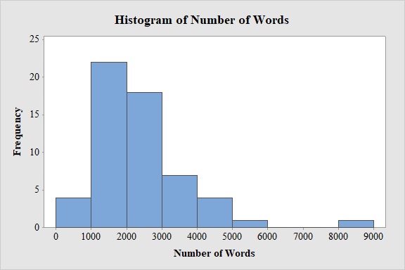
Output obtained from MINITAB software for the number of words spoken is:
The relative frequency distribution for the data is:
| Number of Words | Relative frequency |
| 0-999 | 0.070 |
| 1,000-1,999 | 0.386 |
| 2,000-2,999 | 0.316 |
| 3,000-3,999 | 0.123 |
| 4,000-4,999 | 0.070 |
| 5,000-5,999 | 0.018 |
| 6,000-6,999 | 0.000 |
| 7,000-7,999 | 0.000 |
| 8,000-8,999 | 0.018 |
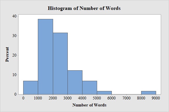
Output obtained from MINITAB software for the number of words spoken is:
Explanation of Solution
Calculation:
Frequency Histogram:
Software procedure:
- Step by step procedure to draw the relative frequency histogram for the number of words spoken using MINITAB software.
- Choose Graph > Histogram.
- Choose Simple.
- Click OK.
- In Graph variables, enter the column of Number of Words.
- In Scale, Choose Y-scale Type as Frequency.
- Click OK.
- Select Edit Scale, Enter 0, 1,000, 2,000, 3,000, 4,000, 5,000, 6,000, 7,000, 8,000, 90,00 in Positions of ticks.
- In Binning, Under Interval Type select Cutpoint and under Interval Definition select Number of intervals as 9 and Cutpoint positions as 0, 1,000, 2,000, 3,000, 4,000, 5,000, 6,000, 7,000, 8,000, 9,000.
- In Labels, Enter 0, 1,000, 2,000, 3,000, 4,000, 5,000, 6,000, 7,000, 8,000, 9,000 in Specified.
- Click OK.
Observation:
From the bar graph, it can be seen that maximum number of words spoken is in the interval 1,000-2,000.
Relative frequency:
Similarly, the relative frequencies for the remaining number of words spoken are obtained below:
| Number of Words | Frequency | Relative frequency |
| 0-999 | 4 | |
| 1,000-1,999 | 22 | |
| 2,000-2,999 | 18 | |
| 3,000-3,999 | 7 | |
| 4,000-4,999 | 4 | |
| 5,000-5,999 | 1 | |
| 6,000-6,999 | 0 | |
| 7,000-7,999 | 0 | |
| 8,000-8,999 | 1 | |
| Total | 57 |
Relative Frequency Histogram:
Software procedure:
- Step by step procedure to draw the relative frequency histogram for the number of words spoken using MINITAB software.
- Choose Graph > Histogram.
- Choose Simple.
- Click OK.
- In Graph variables, enter the column of Number of Words.
- In Scale, Choose Y-scale Type as Percent.
- Click OK.
- Select Edit Scale, Enter 0, 1,000, 2,000, 3,000, 4,000, 5,000, 6,000, 7,000, 8,000 and 9,000 in Positions of ticks.
- In Binning, Under Interval Type select Cutpoint and under Interval Definition select Number of intervals as 9 and Cutpoint positions as 0, 1,000, 2,000, 3,000, 4,000, 5,000, 6,000, 7,000, 8,000 and 9,000.
- In Labels, Enter 0, 1,000, 2,000, 3,000, 4,000, 5,000, 6,000, 7,000, 8,000 and 9,000in Specified.
- Click OK.
Observation:
From the bar graph, it can be seen that maximum number of words spoken is in the interval 1,000-2,000.
h.
Check whether the 9 and 5 classes are reasonable or one choice is much better than the other and explain the reason.
h.
Answer to Problem 31E
Both the 5 and 9 classes are reasonable.
Explanation of Solution
Answer will vary.
The number of classes can be obtained by the following two points:
- The number of classes should be between 5 and 20.
- A larger number of classes will be appropriate for a very large data set.
Here number of classes for the histograms are 5 and 9 respectively. Thus, the number of classes are lies between 5 and 20.
Hence, the both 5 and 9 classes are reasonable.
Want to see more full solutions like this?
Chapter 2 Solutions
Essential Statistics


- For each of the time series, construct a line chart of the data and identify the characteristics of the time series (that is, random, stationary, trend, seasonal, or cyclical). Year Month Rate (%)2009 Mar 8.72009 Apr 9.02009 May 9.42009 Jun 9.52009 Jul 9.52009 Aug 9.62009 Sep 9.82009 Oct 10.02009 Nov 9.92009 Dec 9.92010 Jan 9.82010 Feb 9.82010 Mar 9.92010 Apr 9.92010 May 9.62010 Jun 9.42010 Jul 9.52010 Aug 9.52010 Sep 9.52010 Oct 9.52010 Nov 9.82010 Dec 9.32011 Jan 9.12011 Feb 9.02011 Mar 8.92011 Apr 9.02011 May 9.02011 Jun 9.12011 Jul 9.02011 Aug 9.02011 Sep 9.02011 Oct 8.92011 Nov 8.62011 Dec 8.52012 Jan 8.32012 Feb 8.32012 Mar 8.22012 Apr 8.12012 May 8.22012 Jun 8.22012 Jul 8.22012 Aug 8.12012 Sep 7.82012 Oct…arrow_forwardFor each of the time series, construct a line chart of the data and identify the characteristics of the time series (that is, random, stationary, trend, seasonal, or cyclical). Date IBM9/7/2010 $125.959/8/2010 $126.089/9/2010 $126.369/10/2010 $127.999/13/2010 $129.619/14/2010 $128.859/15/2010 $129.439/16/2010 $129.679/17/2010 $130.199/20/2010 $131.79 a. Construct a line chart of the closing stock prices data. Choose the correct chart below.arrow_forwardFor each of the time series, construct a line chart of the data and identify the characteristics of the time series (that is, random, stationary, trend, seasonal, or cyclical) Date IBM9/7/2010 $125.959/8/2010 $126.089/9/2010 $126.369/10/2010 $127.999/13/2010 $129.619/14/2010 $128.859/15/2010 $129.439/16/2010 $129.679/17/2010 $130.199/20/2010 $131.79arrow_forward
- 1. A consumer group claims that the mean annual consumption of cheddar cheese by a person in the United States is at most 10.3 pounds. A random sample of 100 people in the United States has a mean annual cheddar cheese consumption of 9.9 pounds. Assume the population standard deviation is 2.1 pounds. At a = 0.05, can you reject the claim? (Adapted from U.S. Department of Agriculture) State the hypotheses: Calculate the test statistic: Calculate the P-value: Conclusion (reject or fail to reject Ho): 2. The CEO of a manufacturing facility claims that the mean workday of the company's assembly line employees is less than 8.5 hours. A random sample of 25 of the company's assembly line employees has a mean workday of 8.2 hours. Assume the population standard deviation is 0.5 hour and the population is normally distributed. At a = 0.01, test the CEO's claim. State the hypotheses: Calculate the test statistic: Calculate the P-value: Conclusion (reject or fail to reject Ho): Statisticsarrow_forward21. find the mean. and variance of the following: Ⓒ x(t) = Ut +V, and V indepriv. s.t U.VN NL0, 63). X(t) = t² + Ut +V, U and V incepires have N (0,8) Ut ①xt = e UNN (0162) ~ X+ = UCOSTE, UNNL0, 62) SU, Oct ⑤Xt= 7 where U. Vindp.rus +> ½ have NL, 62). ⑥Xn = ΣY, 41, 42, 43, ... Yn vandom sample K=1 Text with mean zen and variance 6arrow_forwardA psychology researcher conducted a Chi-Square Test of Independence to examine whether there is a relationship between college students’ year in school (Freshman, Sophomore, Junior, Senior) and their preferred coping strategy for academic stress (Problem-Focused, Emotion-Focused, Avoidance). The test yielded the following result: image.png Interpret the results of this analysis. In your response, clearly explain: Whether the result is statistically significant and why. What this means about the relationship between year in school and coping strategy. What the researcher should conclude based on these findings.arrow_forward
- A school counselor is conducting a research study to examine whether there is a relationship between the number of times teenagers report vaping per week and their academic performance, measured by GPA. The counselor collects data from a sample of high school students. Write the null and alternative hypotheses for this study. Clearly state your hypotheses in terms of the correlation between vaping frequency and academic performance. EditViewInsertFormatToolsTable 12pt Paragrapharrow_forwardA smallish urn contains 25 small plastic bunnies – 7 of which are pink and 18 of which are white. 10 bunnies are drawn from the urn at random with replacement, and X is the number of pink bunnies that are drawn. (a) P(X = 5) ≈ (b) P(X<6) ≈ The Whoville small urn contains 100 marbles – 60 blue and 40 orange. The Grinch sneaks in one night and grabs a simple random sample (without replacement) of 15 marbles. (a) The probability that the Grinch gets exactly 6 blue marbles is [ Select ] ["≈ 0.054", "≈ 0.043", "≈ 0.061"] . (b) The probability that the Grinch gets at least 7 blue marbles is [ Select ] ["≈ 0.922", "≈ 0.905", "≈ 0.893"] . (c) The probability that the Grinch gets between 8 and 12 blue marbles (inclusive) is [ Select ] ["≈ 0.801", "≈ 0.760", "≈ 0.786"] . The Whoville small urn contains 100 marbles – 60 blue and 40 orange. The Grinch sneaks in one night and grabs a simple random sample (without replacement) of 15 marbles. (a)…arrow_forwardSuppose an experiment was conducted to compare the mileage(km) per litre obtained by competing brands of petrol I,II,III. Three new Mazda, three new Toyota and three new Nissan cars were available for experimentation. During the experiment the cars would operate under same conditions in order to eliminate the effect of external variables on the distance travelled per litre on the assigned brand of petrol. The data is given as below: Brands of Petrol Mazda Toyota Nissan I 10.6 12.0 11.0 II 9.0 15.0 12.0 III 12.0 17.4 13.0 (a) Test at the 5% level of significance whether there are signi cant differences among the brands of fuels and also among the cars. [10] (b) Compute the standard error for comparing any two fuel brands means. Hence compare, at the 5% level of significance, each of fuel brands II, and III with the standard fuel brand I. [10] �arrow_forward
 Holt Mcdougal Larson Pre-algebra: Student Edition...AlgebraISBN:9780547587776Author:HOLT MCDOUGALPublisher:HOLT MCDOUGAL
 Glencoe Algebra 1, Student Edition, 9780079039897...AlgebraISBN:9780079039897Author:CarterPublisher:McGraw Hill
 Big Ideas Math A Bridge To Success Algebra 1: Stu...AlgebraISBN:9781680331141Author:HOUGHTON MIFFLIN HARCOURTPublisher:Houghton Mifflin Harcourt