Chapter 2, Problem 8RE

a.

To determine

Construct the frequency distribution with approximately eight classes.

Answer to Problem 8RE

The frequency distribution is,

Age	Frequency
10-19	2
20-29	1
30-39	3
40-49	10
50-59	9
60-69	9
70-79	4
80-89	2
Total	40

Explanation of Solution

Calculation:

The given information is that a data representing the age at which the all English and British monarchs died.

Frequency:

The frequencies are calculated by using the tally mark and the range of the data is from 10 to 89.

• Based on the given information, the class intervals are 10-19, 20-29, 30-39, 40-49, 50-59, 60-69, 70-79, 80-89.
• Make a tally mark for each value in the corresponding age class and continue for all values in the data.
• The number of tally marks in each class represents the frequency, f of that class.

Similarly, the frequency of remaining classes for the age is given below:

Age	Tally	Frequency
10-19	$\left|\right|$	2
20-29	$|$	1
30-39	$\left|\right||$	3
40-49	$\bcancel{\left|\right|\left|\right|}\bcancel{\left|\right|\left|\right|}$	10
50-59	$\bcancel{\left|\right|\left|\right|}\left|\right|\left|\right|$	9
60-69	$\bcancel{\left|\right|\left|\right|}\left|\right|\left|\right|$	9
70-79	$\left|\right|\left|\right|$	4
80-89	$\left|\right|$	2
Total		40

b.

To determine

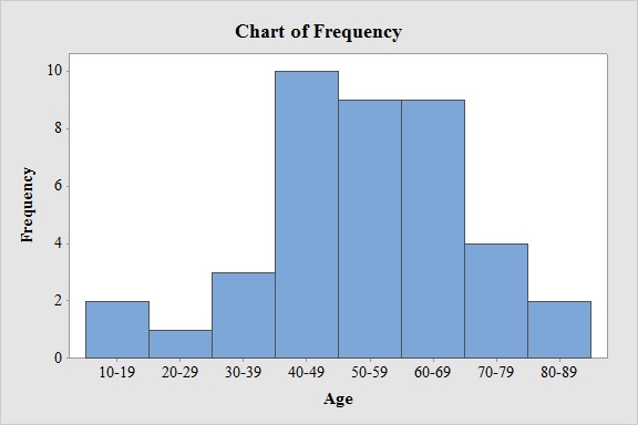
Construct the frequency histogram based on the frequency distribution.

Answer to Problem 8RE

Output obtained from MINITAB software for the ages is:

Explanation of Solution

Calculation:

Frequency Histogram:

Software procedure:

• Step by step procedure to draw the frequency histogram for the ages using MINITAB software.
• Choose Graph > Bar Chart.
• From Bars represent, choose unique values from table.
• Choose Simple.
• Click OK.
• In Graph variables, enter the column of Frequency.
• In Categorical variables, enter the column of Ages.
• Click OK
• Select Edit Scale, Enter 0 in Gap between clusters.

Observation:

From the bar graph, it can be seen that maximum age at death for the monarchs is in the interval 40-49.

c.

To determine

Construct a relative frequency distribution for the data.

Answer to Problem 8RE

The relative frequency distribution for the data is:

Age	Relative frequency
10-19	0.050
20-29	0.025
30-39	0.075
40-49	0.25
50-59	0.225
60-69	0.225
70-79	0.100
80-89	0.050

Explanation of Solution

Calculation:

Relative frequency:

The general formula for the relative frequency is,

$\text{Relative}\text{Frequency = }\frac{\text{Frequency}}{\text{Total frequency}}$

Therefore,

$\begin{array}{c}\text{Relative}\text{Frequency}\text{for the class 10-19}=\frac{2}{40}\\ =0.05\end{array}$

Similarly, the relative frequencies for the remaining ages are obtained below:

Age	Frequency	Relative frequency
10-19	2	$\frac{2}{40}=0.050$
20-29	1	$\frac{1}{40}=0.025$
30-39	3	$\frac{3}{40}=0.075$
40-49	10	$\frac{9}{40}=0.250$
50-59	9	$\frac{9}{40}=0.225$
60-69	9	$\frac{9}{40}=0.225$
70-79	4	$\frac{4}{40}=0.100$
80-89	2	$\frac{2}{40}=0.050$

d.

To determine

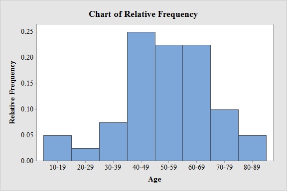
Construct the relative frequency histogram based on the frequency distribution.

Answer to Problem 8RE

Output obtained from MINITAB software for the ages is:

Explanation of Solution

Calculation:

Relative Frequency Histogram:

Software procedure:

• Step by step procedure to draw the relative frequency histogram for the ages using MINITAB software.
• Choose Graph > Bar Chart.
• From Bars represent, choose unique values from table.
• Choose Simple.
• Click OK.
• In Graph variables, enter the column of Relative Frequency.
• In Categorical variables, enter the column of Ages.
• Click OK
• Select Edit Scale, Enter 0 in Gap between clusters.

Observation:

From the bar graph, it can be seen that maximum age at death for the monarchs is in the interval 40-49.