
Essential Statistics
2nd Edition
ISBN: 9781259570643
Author: Navidi
Publisher: MCG
expand_more
expand_more
format_list_bulleted
Concept explainers
Videos
Question
Chapter 2, Problem 1CQ
To determine
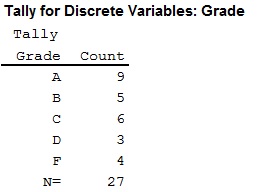
Construct the frequency distribution for the data.
Expert Solution & Answer
Answer to Problem 1CQ
The frequency distribution for the data:
Explanation of Solution
Calculation:
The given information is that a list of letter grades for students in an algebra class, A, B, F, A, C, C, A, B, D, F, D, A, A, B, C, F, B, D, C, A, A, A, F, B, C, A, C.
Frequency:
Software procedure:
- Step by step procedure to obtain a frequency distribution for the data using MINITAB software.
- Choose Stat > Tables>Tally individual Variables.
- Under Variables, choose 'Grades'.
- Under Display, select Counts.
- Click OK.
Want to see more full solutions like this?
Subscribe now to access step-by-step solutions to millions of textbook problems written by subject matter experts!
Students have asked these similar questions
For each of the time series, construct a line chart of the data and identify the characteristics of the time series (that is, random, stationary, trend, seasonal, or cyclical)
Date IBM9/7/2010 $125.959/8/2010 $126.089/9/2010 $126.369/10/2010 $127.999/13/2010 $129.619/14/2010 $128.859/15/2010 $129.439/16/2010 $129.679/17/2010 $130.199/20/2010 $131.79
1. A consumer group claims that the mean annual consumption of cheddar cheese by a person in
the United States is at most 10.3 pounds. A random sample of 100 people in the United States has
a mean annual cheddar cheese consumption of 9.9 pounds. Assume the population standard
deviation is 2.1 pounds. At a = 0.05, can you reject the claim? (Adapted from U.S. Department of
Agriculture)
State the hypotheses:
Calculate the test statistic:
Calculate the P-value:
Conclusion (reject or fail to reject Ho):
2. The CEO of a manufacturing facility claims that the mean workday of the company's assembly
line employees is less than 8.5 hours. A random sample of 25 of the company's assembly line
employees has a mean workday of 8.2 hours. Assume the population standard deviation is 0.5
hour and the population is normally distributed. At a = 0.01, test the CEO's claim.
State the hypotheses:
Calculate the test statistic:
Calculate the P-value:
Conclusion (reject or fail to reject Ho):
Statistics
21.
find the mean.
and
variance of the
following:
Ⓒ x(t) = Ut +V, and V indepriv. s.t
U.VN NL0, 63).
X(t) = t² + Ut +V, U and V incepires have N (0,8)
Ut
①xt = e UNN (0162)
~ X+ = UCOSTE, UNNL0, 62)
SU, Oct
⑤Xt=
7
where U. Vindp.rus
+> ½
have NL, 62).
⑥Xn = ΣY, 41, 42, 43, ... Yn vandom sample
K=1
Text
with mean zen and variance 6
Chapter 2 Solutions
Essential Statistics
Ch. 2.1 - 1. The following table lists the types of aircraft...Ch. 2.1 - Prob. 2CYUCh. 2.1 - Prob. 3CYUCh. 2.1 - Prob. 4CYUCh. 2.1 - Prob. 5ECh. 2.1 - In Exercises 5–8, fill in each blank with the...Ch. 2.1 - Prob. 7ECh. 2.1 -
In Exercises 5–8, fill in each blank with the...Ch. 2.1 - Prob. 9ECh. 2.1 - In Exercises 9–12, determine whether the statement...
Ch. 2.1 - Prob. 11ECh. 2.1 -
In Exercises 9–12, determine whether the...Ch. 2.1 - Prob. 13ECh. 2.1 - 14. The most common blood typing system divides...Ch. 2.1 - 15. Following is a pie chart that presents the...Ch. 2.1 - 16. Student expenses: The following pie chart...Ch. 2.1 - 17. Food sources: The following side-by-side bar...Ch. 2.1 -
18. Super Bowl: The following side-by-side bar...Ch. 2.1 - Prob. 19ECh. 2.1 - 20. Popular video games: The following frequency...Ch. 2.1 - Prob. 21ECh. 2.1 - Prob. 22ECh. 2.1 - Prob. 23ECh. 2.1 - Prob. 24ECh. 2.1 - Prob. 25ECh. 2.1 - 26. How secure is your job? In a survey, employed...Ch. 2.1 - Prob. 27ECh. 2.1 - Prob. 28ECh. 2.1 - Prob. 29ECh. 2.1 - 30. Bought a new car lately? The following table...Ch. 2.1 - Prob. 31ECh. 2.1 - Prob. 32ECh. 2.1 - Prob. 33ECh. 2.1 - Prob. 34ECh. 2.1 - Prob. 35ECh. 2.2 - Using the data in Table 2.7, construct a frequency...Ch. 2.2 - Prob. 2CYUCh. 2.2 - Prob. 3CYUCh. 2.2 - Prob. 4CYUCh. 2.2 - Prob. 5ECh. 2.2 -
In Exercises 5-8, fill in each blank with the...Ch. 2.2 - Prob. 7ECh. 2.2 - Prob. 8ECh. 2.2 - Prob. 9ECh. 2.2 - Prob. 10ECh. 2.2 - Prob. 11ECh. 2.2 - In Exercises 9-12, determine whether the statement...Ch. 2.2 - Prob. 13ECh. 2.2 - In Exercises 13–16, classify the histogram as...Ch. 2.2 - Prob. 15ECh. 2.2 - In Exercises 13–16, classify the histogram as...Ch. 2.2 - In Exercises 17 and 18, classify the histogram as...Ch. 2.2 - In Exercises 17 and 18, classify the histogram as...Ch. 2.2 - Prob. 19ECh. 2.2 - 20. Trained rats: Forty rats were trained to run a...Ch. 2.2 - 21. Interpret histogram: The following histogram...Ch. 2.2 - Prob. 22ECh. 2.2 - Prob. 23ECh. 2.2 - Skewed which way? For which of the following data...Ch. 2.2 - Prob. 25ECh. 2.2 - 26. Batting average: The following frequency...Ch. 2.2 - Prob. 27ECh. 2.2 - 28. Murder, she wrote: The following frequency...Ch. 2.2 - BMW prices: The following table presents the...Ch. 2.2 - Geysers: The geyser Old Faithful in Yellowstone...Ch. 2.2 - Prob. 31ECh. 2.2 - Internet radio: The following table presents the...Ch. 2.2 - Prob. 33ECh. 2.2 - Prob. 34ECh. 2.2 - Prob. 35ECh. 2.2 - Prob. 36ECh. 2.2 - 37. Silver ore: The following histogram presents...Ch. 2.2 - Classes of differing widths: Consider the...Ch. 2.3 - Weights of college students: The following table...Ch. 2.3 - Prob. 2CYUCh. 2.3 - Prob. 3ECh. 2.3 - Prob. 4ECh. 2.3 - In Exercises 3–6, fill in each blank with the...Ch. 2.3 - Prob. 6ECh. 2.3 - Prob. 7ECh. 2.3 - Prob. 8ECh. 2.3 - Prob. 9ECh. 2.3 - Prob. 10ECh. 2.3 - Prob. 11ECh. 2.3 - Prob. 12ECh. 2.3 - Prob. 13ECh. 2.3 - 14. List the data in the following stem-and-leaf...Ch. 2.3 - Prob. 15ECh. 2.3 - Prob. 16ECh. 2.3 - BMW prices: The following table presents the...Ch. 2.3 - How’s the weather? The following table presents...Ch. 2.3 - Prob. 19ECh. 2.3 - Prob. 20ECh. 2.3 - Tennis and golf: Following are the ages of the...Ch. 2.3 - Prob. 22ECh. 2.3 - Prob. 23ECh. 2.3 - 24. Safety first: Following are the numbers of...Ch. 2.3 - Prob. 25ECh. 2.3 - Prob. 26ECh. 2.3 - Prob. 27ECh. 2.3 - Prob. 28ECh. 2.3 - Prob. 29ECh. 2.3 - 30. Going for gold: The following time-series plot...Ch. 2.3 - Prob. 31ECh. 2.3 - Prob. 32ECh. 2.3 - Prob. 33ECh. 2.3 - 34. Arctic ice sheet: The following table presents...Ch. 2.3 - Prob. 35ECh. 2.4 - The population of country A is twice as large as...Ch. 2.4 - Prob. 2CYUCh. 2.4 - Prob. 3ECh. 2.4 - Prob. 4ECh. 2.4 - Prob. 5ECh. 2.4 - Prob. 6ECh. 2.4 - Prob. 7ECh. 2.4 - Prob. 8ECh. 2.4 - Prob. 9ECh. 2.4 - Prob. 10ECh. 2.4 - Prob. 11ECh. 2.4 - Prob. 12ECh. 2.4 - College degrees: Both of the following time-series...Ch. 2.4 - Food expenditures: Both of the following...Ch. 2.4 - Prob. 15ECh. 2 - Prob. 1CQCh. 2 - Prob. 2CQCh. 2 - Prob. 3CQCh. 2 - Prob. 4CQCh. 2 - Prob. 5CQCh. 2 - 6. True or false: A histogram can have more than...Ch. 2 - Prob. 7CQCh. 2 - Prob. 8CQCh. 2 - Prob. 9CQCh. 2 - Prob. 10CQCh. 2 - Prob. 11CQCh. 2 - Prob. 12CQCh. 2 - Prob. 13CQCh. 2 - Prob. 14CQCh. 2 - Prob. 15CQCh. 2 - Prob. 1RECh. 2 - Prob. 2RECh. 2 - Prob. 3RECh. 2 - Prob. 4RECh. 2 - Prob. 5RECh. 2 - Prob. 6RECh. 2 - Prob. 7RECh. 2 - Prob. 8RECh. 2 - Prob. 9RECh. 2 - Prob. 10RECh. 2 - Prob. 11RECh. 2 - Prob. 12RECh. 2 - Prob. 13RECh. 2 - Prob. 14RECh. 2 - Prob. 15RECh. 2 - Prob. 1WAICh. 2 - Prob. 2WAICh. 2 - Prob. 3WAICh. 2 - Prob. 4WAICh. 2 - Prob. 1CSCh. 2 - Prob. 2CSCh. 2 - In the chapter introduction, we presented gas...Ch. 2 - Prob. 4CSCh. 2 - Prob. 5CSCh. 2 - Prob. 6CSCh. 2 - Prob. 7CSCh. 2 - Prob. 8CSCh. 2 - Prob. 9CS
Knowledge Booster


Learn more about
Need a deep-dive on the concept behind this application? Look no further. Learn more about this topic, statistics and related others by exploring similar questions and additional content below.Similar questions
- A psychology researcher conducted a Chi-Square Test of Independence to examine whether there is a relationship between college students’ year in school (Freshman, Sophomore, Junior, Senior) and their preferred coping strategy for academic stress (Problem-Focused, Emotion-Focused, Avoidance). The test yielded the following result: image.png Interpret the results of this analysis. In your response, clearly explain: Whether the result is statistically significant and why. What this means about the relationship between year in school and coping strategy. What the researcher should conclude based on these findings.arrow_forwardA school counselor is conducting a research study to examine whether there is a relationship between the number of times teenagers report vaping per week and their academic performance, measured by GPA. The counselor collects data from a sample of high school students. Write the null and alternative hypotheses for this study. Clearly state your hypotheses in terms of the correlation between vaping frequency and academic performance. EditViewInsertFormatToolsTable 12pt Paragrapharrow_forwardA smallish urn contains 25 small plastic bunnies – 7 of which are pink and 18 of which are white. 10 bunnies are drawn from the urn at random with replacement, and X is the number of pink bunnies that are drawn. (a) P(X = 5) ≈ (b) P(X<6) ≈ The Whoville small urn contains 100 marbles – 60 blue and 40 orange. The Grinch sneaks in one night and grabs a simple random sample (without replacement) of 15 marbles. (a) The probability that the Grinch gets exactly 6 blue marbles is [ Select ] ["≈ 0.054", "≈ 0.043", "≈ 0.061"] . (b) The probability that the Grinch gets at least 7 blue marbles is [ Select ] ["≈ 0.922", "≈ 0.905", "≈ 0.893"] . (c) The probability that the Grinch gets between 8 and 12 blue marbles (inclusive) is [ Select ] ["≈ 0.801", "≈ 0.760", "≈ 0.786"] . The Whoville small urn contains 100 marbles – 60 blue and 40 orange. The Grinch sneaks in one night and grabs a simple random sample (without replacement) of 15 marbles. (a)…arrow_forward
- Suppose an experiment was conducted to compare the mileage(km) per litre obtained by competing brands of petrol I,II,III. Three new Mazda, three new Toyota and three new Nissan cars were available for experimentation. During the experiment the cars would operate under same conditions in order to eliminate the effect of external variables on the distance travelled per litre on the assigned brand of petrol. The data is given as below: Brands of Petrol Mazda Toyota Nissan I 10.6 12.0 11.0 II 9.0 15.0 12.0 III 12.0 17.4 13.0 (a) Test at the 5% level of significance whether there are signi cant differences among the brands of fuels and also among the cars. [10] (b) Compute the standard error for comparing any two fuel brands means. Hence compare, at the 5% level of significance, each of fuel brands II, and III with the standard fuel brand I. [10] �arrow_forwardBusiness discussarrow_forwardWhat would you say about a set of quantitative bivariate data whose linear correlation is -1? What would a scatter diagram of the data look like? (5 points)arrow_forward
- Business discussarrow_forwardAnalyze the residuals of a linear regression model and select the best response. yes, the residual plot does not show a curve no, the residual plot shows a curve yes, the residual plot shows a curve no, the residual plot does not show a curve I answered, "No, the residual plot shows a curve." (and this was incorrect). I am not sure why I keep getting these wrong when the answer seems obvious. Please help me understand what the yes and no references in the answer.arrow_forwarda. Find the value of A.b. Find pX(x) and py(y).c. Find pX|y(x|y) and py|X(y|x)d. Are x and y independent? Why or why not?arrow_forward
- Analyze the residuals of a linear regression model and select the best response.Criteria is simple evaluation of possible indications of an exponential model vs. linear model) no, the residual plot does not show a curve yes, the residual plot does not show a curve yes, the residual plot shows a curve no, the residual plot shows a curve I selected: yes, the residual plot shows a curve and it is INCORRECT. Can u help me understand why?arrow_forwardYou have been hired as an intern to run analyses on the data and report the results back to Sarah; the five questions that Sarah needs you to address are given below. please do it step by step on excel Does there appear to be a positive or negative relationship between price and screen size? Use a scatter plot to examine the relationship. Determine and interpret the correlation coefficient between the two variables. In your interpretation, discuss the direction of the relationship (positive, negative, or zero relationship). Also discuss the strength of the relationship. Estimate the relationship between screen size and price using a simple linear regression model and interpret the estimated coefficients. (In your interpretation, tell the dollar amount by which price will change for each unit of increase in screen size). Include the manufacturer dummy variable (Samsung=1, 0 otherwise) and estimate the relationship between screen size, price and manufacturer dummy as a multiple…arrow_forwardHere is data with as the response variable. x y54.4 19.124.9 99.334.5 9.476.6 0.359.4 4.554.4 0.139.2 56.354 15.773.8 9-156.1 319.2Make a scatter plot of this data. Which point is an outlier? Enter as an ordered pair, e.g., (x,y). (x,y)= Find the regression equation for the data set without the outlier. Enter the equation of the form mx+b rounded to three decimal places. y_wo= Find the regression equation for the data set with the outlier. Enter the equation of the form mx+b rounded to three decimal places. y_w=arrow_forward
arrow_back_ios
SEE MORE QUESTIONS
arrow_forward_ios
Recommended textbooks for you
 MATLAB: An Introduction with ApplicationsStatisticsISBN:9781119256830Author:Amos GilatPublisher:John Wiley & Sons Inc
 Probability and Statistics for Engineering and th...StatisticsISBN:9781305251809Author:Jay L. DevorePublisher:Cengage Learning
 Statistics for The Behavioral Sciences (MindTap C...StatisticsISBN:9781305504912Author:Frederick J Gravetter, Larry B. WallnauPublisher:Cengage Learning
 Elementary Statistics: Picturing the World (7th E...StatisticsISBN:9780134683416Author:Ron Larson, Betsy FarberPublisher:PEARSON
 The Basic Practice of StatisticsStatisticsISBN:9781319042578Author:David S. Moore, William I. Notz, Michael A. FlignerPublisher:W. H. Freeman
 Introduction to the Practice of StatisticsStatisticsISBN:9781319013387Author:David S. Moore, George P. McCabe, Bruce A. CraigPublisher:W. H. Freeman
MATLAB: An Introduction with Applications
Statistics
ISBN:9781119256830
Author:Amos Gilat
Publisher:John Wiley & Sons Inc
Probability and Statistics for Engineering and th...
Statistics
ISBN:9781305251809
Author:Jay L. Devore
Publisher:Cengage Learning
Statistics for The Behavioral Sciences (MindTap C...
Statistics
ISBN:9781305504912
Author:Frederick J Gravetter, Larry B. Wallnau
Publisher:Cengage Learning
Elementary Statistics: Picturing the World (7th E...
Statistics
ISBN:9780134683416
Author:Ron Larson, Betsy Farber
Publisher:PEARSON
The Basic Practice of Statistics
Statistics
ISBN:9781319042578
Author:David S. Moore, William I. Notz, Michael A. Fligner
Publisher:W. H. Freeman
Introduction to the Practice of Statistics
Statistics
ISBN:9781319013387
Author:David S. Moore, George P. McCabe, Bruce A. Craig
Publisher:W. H. Freeman
The Shape of Data: Distributions: Crash Course Statistics #7; Author: CrashCourse;https://www.youtube.com/watch?v=bPFNxD3Yg6U;License: Standard YouTube License, CC-BY
Shape, Center, and Spread - Module 20.2 (Part 1); Author: Mrmathblog;https://www.youtube.com/watch?v=COaid7O_Gag;License: Standard YouTube License, CC-BY
Shape, Center and Spread; Author: Emily Murdock;https://www.youtube.com/watch?v=_YyW0DSCzpM;License: Standard Youtube License