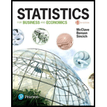
Statistics for Business and Economics (13th Edition)
13th Edition
ISBN: 9780134506593
Author: James T. McClave, P. George Benson, Terry Sincich
Publisher: PEARSON
expand_more
expand_more
format_list_bulleted
Concept explainers
Textbook Question
Chapter 14.9, Problem 14.53ACB
Predicting presidential elections. Refer to the Political Analysis (Vol. 17, 2009) study on predicting presidential elections, Exercise 14.44 (p. 14-37). Recall that a regression model with five independent variables was fit to data collected for n = 24 election years in order to predict Yt = percentage of the two-party vote won by the incumbent party’s candidate in election year t. The Durbin-Watson d-statistic for the model was reported as d = 1. 77. Is there evidence (at α = .05) of
Expert Solution & Answer
Want to see the full answer?
Check out a sample textbook solution
Students have asked these similar questions
The college hiking club is having a fundraiser to buy new equipment for fall and winter outings. The club is selling Chinese fortune cookies at a price of $2 per cookie. Each cookie contains a piece of paper with a different number written on it. A random drawing will determine which number is the winner of a dinner for two at a local Chinese restaurant. The dinner is valued at $32. Since fortune cookies are donated to the club, we can ignore the cost of the cookies. The club sold 718 cookies before the drawing. Lisa bought 13 cookies. Lisa's expected earnings can be found by multiplying the value of the dinner by the probability that she will win. What are Lisa's expected earnings? Round your answer to the nearest cent.
The Honolulu Advertiser stated that in Honolulu there was an average of 659 burglaries per 400,000 households in a given year. In the Kohola Drive neighborhood there are 321 homes. Let r be the number of homes that will be burglarized in a year. Use the formula for Poisson distribution. What is the value of p, the probability of success, to four decimal places?
The college hiking club is having a fundraiser to buy new equipment for fall and winter outings. The club is selling Chinese fortune cookies at a price of $2 per cookie. Each cookie contains a piece of paper with a different number written on it. A random drawing will determine which number is the winner of a dinner for two at a local Chinese restaurant. The dinner is valued at $32. Since fortune cookies are donated to the club, we can ignore the cost of the cookies. The club sold 718 cookies before the drawing. Lisa bought 13 cookies. Lisa's expected earnings can be found by multiplying the value of the dinner by the probability that she will win. What are Lisa's expected earnings? Round your answer to the nearest cent.
Chapter 14 Solutions
Statistics for Business and Economics (13th Edition)
Ch. 14.1 - Explain in words how to construct a simple index.Ch. 14.1 - Explain in words how to calculate the following...Ch. 14.1 - Explain in words the difference between Laspeyres...Ch. 14.1 - The table below gives the prices for three...Ch. 14.1 - Refer to Exercise 14.4. The next table gives the...Ch. 14.1 - Annual median family income. The table below lists...Ch. 14.1 - Annual U.S. craft beer production. While overall...Ch. 14.1 - Quarterly single-family housing starts. The...Ch. 14.1 - Spot price of natural gas. The table shown in the...Ch. 14.1 - Employment in farm and nonfarm categories....
Ch. 14.1 - GOP personal consumption expenditures. The gross...Ch. 14.1 - GDP personal consumption expenditures (contd)....Ch. 14.1 - Weekly earnings for workers. The table in the next...Ch. 14.1 - Production and price of metals. The level or price...Ch. 14.2 - Describe the effect of selecting an exponential...Ch. 14.2 - A monthly time series is shown in the table to the...Ch. 14.2 - Annual U.S. craft beer production. Refer to the...Ch. 14.2 - Foreign fish production. Overfishing and pollution...Ch. 14.2 - Yearly price of gold. The price of gold is used by...Ch. 14.2 - Personal consumption in transportation. There has...Ch. 14.2 - OPEC crude oil imports. The data in the table...Ch. 14.2 - SP 500 Stock Index. Standard Poors 500 Composite...Ch. 14.5 - How does the choice of the smoothing constant w...Ch. 14.5 - Refer to Exercise 14.4 (p. 14-9). The table with...Ch. 14.5 - Annual U.S. craft beer production. Refer to...Ch. 14.5 - Quarterly single-family housing starts. Refer to...Ch. 14.5 - Consumer Price Index. The CPI measures the...Ch. 14.5 - OPEC crude oil imports. Refer to the annual OPEC...Ch. 14.5 - SP 500 Stock Index. Refer to the quarterly...Ch. 14.5 - SP 500 Stock Index (contd). Refer to Exercise...Ch. 14.5 - Monthly gold prices. The fluctuation of gold...Ch. 14.6 - Annual U.S. craft beer production. Refer to the...Ch. 14.6 - Annual U.S. craft beer production (contd). Refer...Ch. 14.6 - SP 500 Stock Index. Refer to your exponential...Ch. 14.6 - SP 500 Stock Index (contd). Refer to your Holt...Ch. 14.6 - Monthly gold prices. Refer to the monthly gold...Ch. 14.6 - US school enrollments. The next table reports...Ch. 14.8 - The annual price of a finished product (in cents...Ch. 14.8 - Retail sales in Quarters 14 over a 10-year period...Ch. 14.8 - What advantage do regression forecasts have over...Ch. 14.8 - Mortgage interest rates. The level at which...Ch. 14.8 - Price of natural gas. Refer to Exercise 14.9 (p....Ch. 14.8 - A gasoline tax on carbon emissions. In an effort...Ch. 14.8 - Predicting presidential elections. Researchers at...Ch. 14.8 - Life insurance policies in force. The table below...Ch. 14.8 - Graphing calculator sales. The next table presents...Ch. 14.8 - Prob. 14.47ACICh. 14.9 - Define autocorrelation. Explain why it is...Ch. 14.9 - For each case, indicate the decision regarding the...Ch. 14.9 - What do the following Durbin-Watson statistics...Ch. 14.9 - Company donations to charity. Refer to the Journal...Ch. 14.9 - Forecasting monthly car and truck sales. Forecasts...Ch. 14.9 - Predicting presidential elections. Refer to the...Ch. 14.9 - Mortgage interest rates. Refer to the data on...Ch. 14.9 - Price of natural gas. Refer to the annual data on...Ch. 14.9 - Life insurance policies in force. Refer to the...Ch. 14.9 - Modeling the deposit share of a retail bank....Ch. 14 - Insured Social Security workers. Workers insured...Ch. 14 - Insured Social Security workers (contd). Refer to...Ch. 14 - Retail prices of food items. In 1990, the average...Ch. 14 - Demand for emergency room services. With the...Ch. 14 - Mortgage interest rates. Refer to the annual...Ch. 14 - Price of Abbott Labs stock. The yearly closing...Ch. 14 - Price o f Abbott Labs stock (contd). Refer to...Ch. 14 - Prob. 14.65ACICh. 14 - Prob. 14.66ACICh. 14 - Quarterly GOP values (contd). Refer to Exercise...Ch. 14 - Prob. 14.68ACICh. 14 - Prob. 14.69ACICh. 14 - Prob. 14.70ACICh. 14 - IBM stock prices. Refer to Example 14.1 (p. 14-5)...Ch. 14 - Prob. 14.72ACI
Knowledge Booster
Learn more about
Need a deep-dive on the concept behind this application? Look no further. Learn more about this topic, statistics and related others by exploring similar questions and additional content below.Similar questions
- What was the age distribution of nurses in Great Britain at the time of Florence Nightingale? Thanks to Florence Nightingale and the British census of 1851, we have the following information (based on data from the classic text Notes on Nursing, by Florence Nightingale). Note: In 1851 there were 25,466 nurses in Great Britain. Furthermore, Nightingale made a strict distinction between nurses and domestic servants. Use a histogram and graph the probability distribution. Using the graph of the probability distribution determine the probability that a British nurse selected at random in 1851 would be 40 years of age or older. Round your answer to nearest thousandth. Age range (yr) 20–29 30–39 40–49 50–59 60–69 70–79 80+ Midpoint (x) 24.5 34.5 44.5 54.5 64.5 74.5 84.5 Percent of nurses 5.7% 9.7% 19.5% 29.2% 25.0% 9.1% 1.8%arrow_forwardWhat was the age distribution of nurses in Great Britain at the time of Florence Nightingale? Thanks to Florence Nightingale and the British census of 1851, we have the following information (based on data from the classic text Notes on Nursing, by Florence Nightingale). Note: In 1851 there were 25,466 nurses in Great Britain. Furthermore, Nightingale made a strict distinction between nurses and domestic servants. Use a histogram and graph the probability distribution. Using the graph of the probability distribution determine the probability that a British nurse selected at random in 1851 would be 40 years of age or older. Round your answer to nearest thousandth. Age range (yr) 20–29 30–39 40–49 50–59 60–69 70–79 80+ Midpoint (x) 24.5 34.5 44.5 54.5 64.5 74.5 84.5 Percent of nurses 5.7% 9.7% 19.5% 29.2% 25.0% 9.1% 1.8%arrow_forwardThere are 4 radar stations and the probability of a single radar station detecting an enemy plane is 0.55. Make a histogram for the probability distribution.arrow_forward
- show all stepsarrow_forwardMost people know that the probability of getting a head when you flip a fair coin is . You want to use the relative frequency of the event to show that the probability is . How many times should you simulate flipping the coin in the experiment? Would it be better to use 300 trials or 3000 trials? Explain.arrow_forwardThe qualified applicant pool for eight management trainee positions consists of ten women and six men. How many different groups of applicants can be selected for the positionsarrow_forward
- You want to make a salad from whatever vegetable you have in the fridge. You have seven different tomatoes. There are 2 red tomatoes, 4 yellow tomatoes, and one black tomato in the fridge. You have three different bell peppers. There is 1 red pepper, 1 yellow pepper, and 1 green pepper. What is the probability of randomly choosing a vegetable and getting a red tomato, and a green pepper? Round your answer to four decimal places.arrow_forwarduppose automobile insurance companies gave annual premiums for top-rated companies in several states. The figure below shows box plots for the annual premium for urban customers in three states. Which state offers the lowest premium? Which state offers the highest premium?arrow_forwardWing Foot is a shoe franchise commonly found in shopping centers across the United States. Wing Foot knows that its stores will not show a profit unless they gross over $940,000 per year. Let A be the event that a new Wing Foot store grosses over $940,000 its first year. Let B be the event that a store grosses over $940,000 its second year. Wing Foot has an administrative policy of closing a new store if it does not show a profit in either of the first two years. Assume that the accounting office at Wing Foot provided the following information: 58% of all Wing Foot stores show a profit the first year; 72% of all Wing Foot store show a profit the second year (this includes stores that did not show a profit the first year); however, 86% of Wing Foot stores that showed a profit the first year also showed a profit the second year. Compute P(B|Ac). Round your answer to the nearest hundredth.arrow_forward
- You draw two cards from a standard deck of 52 cards, but before you draw the second card, you put the first one back and reshuffle the deck. If you get a3on the first card, find the probability of drawing a 3 for the second card.arrow_forwardDo bonds reduce the overall risk of an investment portfolio? Let x be a random variable representing annual percent return for the Vanguard Total Stock Index (all Stocks). Let y be a random variable representing annual return for the Vanguard Balanced Index (60% stock and 40% bond). For the past several years, assume the following data. Compute the coefficient of variation for each fund. Round your answers to the nearest tenth. x: 14 0 37 21 35 23 24 -14 -14 -17 y: 8 -2 29 17 22 17 17 -2 -3 -8arrow_forwardWhat percentage of the general U.S. population have bachelor's degrees? Suppose that the Statistical Abstract of the United States, 120th Edition, gives the following percentage of bachelor’s degrees by state. For convenience, the data are sorted in increasing order. 17 18 18 18 19 20 20 20 21 21 21 21 21 22 22 22 22 22 23 23 24 24 24 24 24 25 25 25 25 26 26 26 26 26 26 27 27 27 28 28 28 29 29 31 31 32 32 34 35 38 Illinois has a bachelor's degree percentage rate of about 18%. Into what quartile does this rate fall?arrow_forward
arrow_back_ios
SEE MORE QUESTIONS
arrow_forward_ios
Recommended textbooks for you
 Big Ideas Math A Bridge To Success Algebra 1: Stu...AlgebraISBN:9781680331141Author:HOUGHTON MIFFLIN HARCOURTPublisher:Houghton Mifflin Harcourt
 Glencoe Algebra 1, Student Edition, 9780079039897...AlgebraISBN:9780079039897Author:CarterPublisher:McGraw Hill
 College AlgebraAlgebraISBN:9781305115545Author:James Stewart, Lothar Redlin, Saleem WatsonPublisher:Cengage Learning
 Linear Algebra: A Modern IntroductionAlgebraISBN:9781285463247Author:David PoolePublisher:Cengage Learning

Big Ideas Math A Bridge To Success Algebra 1: Stu...
Algebra
ISBN:9781680331141
Author:HOUGHTON MIFFLIN HARCOURT
Publisher:Houghton Mifflin Harcourt

Glencoe Algebra 1, Student Edition, 9780079039897...
Algebra
ISBN:9780079039897
Author:Carter
Publisher:McGraw Hill

College Algebra
Algebra
ISBN:9781305115545
Author:James Stewart, Lothar Redlin, Saleem Watson
Publisher:Cengage Learning


Linear Algebra: A Modern Introduction
Algebra
ISBN:9781285463247
Author:David Poole
Publisher:Cengage Learning
Correlation Vs Regression: Difference Between them with definition & Comparison Chart; Author: Key Differences;https://www.youtube.com/watch?v=Ou2QGSJVd0U;License: Standard YouTube License, CC-BY
Correlation and Regression: Concepts with Illustrative examples; Author: LEARN & APPLY : Lean and Six Sigma;https://www.youtube.com/watch?v=xTpHD5WLuoA;License: Standard YouTube License, CC-BY