
Thinking Like an Engineer: An Active Learning Approach (4th Edition)
4th Edition
ISBN: 9780134639673
Author: Elizabeth A. Stephan, David R. Bowman, William J. Park, Benjamin L. Sill, Matthew W. Ohland
Publisher: PEARSON
expand_more
expand_more
format_list_bulleted
Concept explainers
Textbook Question
Chapter 13, Problem 11ICA
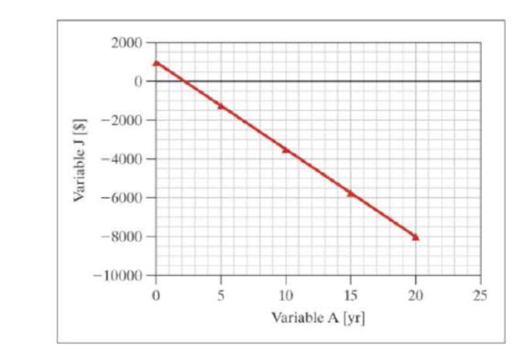
The following instructions will apply to ICA 13-10 to 13-21, for the preceding graph, identify:
- whether this model is linear, power, exponential, or none of those options,
- what is the equation of the line shown in the graph, and
- the units of each value represented in the equation of the line.
ICA 13-11
Expert Solution & Answer
Want to see the full answer?
Check out a sample textbook solution
Students have asked these similar questions
A vessel loads 680 t fuel between forward and aft deep tanks. centre of gravity of forward tank is 24m forward of ships COG. centre to centre between tanks is 42 m. how much in each tank to keep trim the same
Beam of a vessel is 11% its length. Cw =0.72. When floating in SW of relative denisity 1.03, TPC is 0.35t greater than in freshwater. Find the length of the ship
An inclining experiment was carried out on a ship of 4000tonne displacement, when masses of 6 tonne were moved transverselythrough 13.5 m. The deflections of a 7.5 m pendulurnwere 81, 78, 85, 83, 79, 82, 84 and 80 mm respectively.Caiculate the metacentric height.
Chapter 13 Solutions
Thinking Like an Engineer: An Active Learning Approach (4th Edition)
Ch. 13.2 - An unknown amount of oxygen, kept in 8 piston-type...Ch. 13.2 - The data shown graphically in the figure describe...Ch. 13.5 - Prob. 3CCCh. 13.5 - Prob. 4CCCh. 13 - Capillary action draws liquid up a narrow tube...Ch. 13 - Several reactions are carried out in a closed...Ch. 13 - An environmental engineer has obtained a bacteria...Ch. 13 - In a turbine a device used for mixing the power...Ch. 13 - Being quite interested in obsolete electronics,...Ch. 13 - Referring to the previous ICA 13-5, Angus is also...
Ch. 13 - Prob. 7ICACh. 13 - The following instructions apply to ICA 13-7 to...Ch. 13 - The following instructions apply to ICA 13-7 to...Ch. 13 - The following instructions will apply to ICA 13-10...Ch. 13 - The following instructions will apply to ICA 13-10...Ch. 13 - The following instructions will apply to ICA 13-10...Ch. 13 - The following instructions will apply to ICA 13-10...Ch. 13 - The following instructions will apply to ICA 13-10...Ch. 13 - The following instructions will apply to ICA 13-10...Ch. 13 - The following instructions will apply to ICA 13-10...Ch. 13 - The following instructions will apply to ICA 13-10...Ch. 13 - The following instructions will apply to ICA 13-10...Ch. 13 - Prob. 21ICACh. 13 - As a reminder, the Reynolds number is discussed in...Ch. 13 - As a reminder, the Reynolds number is discussed in...Ch. 13 - An environmental engineer has obtained a bacteria...Ch. 13 - An environmental engineer has obtained a bacteria...Ch. 13 - An environmental engineer has obtained a bacteria...Ch. 13 - A growing field of inquiry that poses both great...Ch. 13 - If an object is heated, the temperature of the...Ch. 13 - The Volcanic Explosivity Index (VEI) is based...Ch. 13 - You are an engineer for a plastics manufacturing...Ch. 13 - A Pitot tube is a device used to measure the...Ch. 13 - As part of an electronic music synthesizer you...Ch. 13 - The following data were collected during testing...Ch. 13 - The relationship of the power required by a...Ch. 13 - When a fluid flows around an object, it creates a...
Knowledge Booster
Learn more about
Need a deep-dive on the concept behind this application? Look no further. Learn more about this topic, mechanical-engineering and related others by exploring similar questions and additional content below.Similar questions
- A ship of 10 000 tonne displacement has a waterplanearea of 1300 m2. The ship loads in water of 1.010 t/m3 andmoves into water of 1.026 t/m3. Find the change in meandraughtarrow_forwardA ship of 7000 tonne displacement has a waterplane areaof 1500 m2. In passing from sea water into river water of1005 kg/m3 there is an increase in draught of 10 cm. Find the Idensity of the sea water.arrow_forwardA ship has 300 tonne of cargo in the hold, 24 m forward ofmidships. The displacement of the vessel is 6000 tonne and its centre of gravity is 1.2 m forward of midships.Find the new position of the centre of gravity if this cargo ismoved to an after hold, 40 m from midshipsarrow_forward
- Sketch and describe how ships are supported in dry dock. When and where does the greatest amount of stresses occur?arrow_forwardSketch and desribe a balanced rudder and how it is suspendedarrow_forwardA ship 140 m long and 18 m beam floats at a draught of9 m. The immersed cross-sectionai areas at equai intervais are 5,60, 116, 145, 152, 153, 153, 151, 142, 85 and 0 m2 respectively.Calculate:(a) displacement(b) block coefficient(c) midship section area coefficient(d) prismatic coefficient.arrow_forward
- A steamer has waterplane area 1680m2 recorded in water with relative denisty 1.013. Displacement = 1200 t, calculate difference in draught in salwater reltive denisity 1.025.arrow_forwardrelative velocity 11.72 m/s is correct, need help finding the angle pleasearrow_forwardDetermine the distance between the two automobiles 2 s after A has passed through the intersection.arrow_forward
- A box barge 65 m long and 12 m wide floats at a draught of5.5 m in sea water. Calculate:(a) the displacement of the barge,(b) its draught in fresh waterarrow_forwardwhat is the angle of the velocity of block B? velocity is 7.46 in/s Determine the acceleration and angle of block B. (Round the acceleration value to three decimal places.)arrow_forwardDetermine the relative velocity of B with respect to A.arrow_forward
arrow_back_ios
SEE MORE QUESTIONS
arrow_forward_ios
Recommended textbooks for you
 Elements Of ElectromagneticsMechanical EngineeringISBN:9780190698614Author:Sadiku, Matthew N. O.Publisher:Oxford University Press
 Mechanics of Materials (10th Edition)Mechanical EngineeringISBN:9780134319650Author:Russell C. HibbelerPublisher:PEARSON
 Thermodynamics: An Engineering ApproachMechanical EngineeringISBN:9781259822674Author:Yunus A. Cengel Dr., Michael A. BolesPublisher:McGraw-Hill Education
 Control Systems EngineeringMechanical EngineeringISBN:9781118170519Author:Norman S. NisePublisher:WILEY
 Mechanics of Materials (MindTap Course List)Mechanical EngineeringISBN:9781337093347Author:Barry J. Goodno, James M. GerePublisher:Cengage Learning
 Engineering Mechanics: StaticsMechanical EngineeringISBN:9781118807330Author:James L. Meriam, L. G. Kraige, J. N. BoltonPublisher:WILEY

Elements Of Electromagnetics
Mechanical Engineering
ISBN:9780190698614
Author:Sadiku, Matthew N. O.
Publisher:Oxford University Press

Mechanics of Materials (10th Edition)
Mechanical Engineering
ISBN:9780134319650
Author:Russell C. Hibbeler
Publisher:PEARSON

Thermodynamics: An Engineering Approach
Mechanical Engineering
ISBN:9781259822674
Author:Yunus A. Cengel Dr., Michael A. Boles
Publisher:McGraw-Hill Education

Control Systems Engineering
Mechanical Engineering
ISBN:9781118170519
Author:Norman S. Nise
Publisher:WILEY

Mechanics of Materials (MindTap Course List)
Mechanical Engineering
ISBN:9781337093347
Author:Barry J. Goodno, James M. Gere
Publisher:Cengage Learning

Engineering Mechanics: Statics
Mechanical Engineering
ISBN:9781118807330
Author:James L. Meriam, L. G. Kraige, J. N. Bolton
Publisher:WILEY
Introduction to Diffusion in Solids; Author: Engineering and Design Solutions;https://www.youtube.com/watch?v=K_1QmKJvNjc;License: Standard youtube license