
Concept explainers
The paper “Less Air Pollution Leads to Rapid Reduction of Airway Inflammation and Improved Airway
The authors of the paper used paired t tests to determine that there was a significant difference in the urban and rural means for each of these three measures. One of these tests resulted in a P-value less than 0.001, one resulted in a P-value between 0.001 and 0.01, and one resulted in a P-value between 0.01 and 0.05.
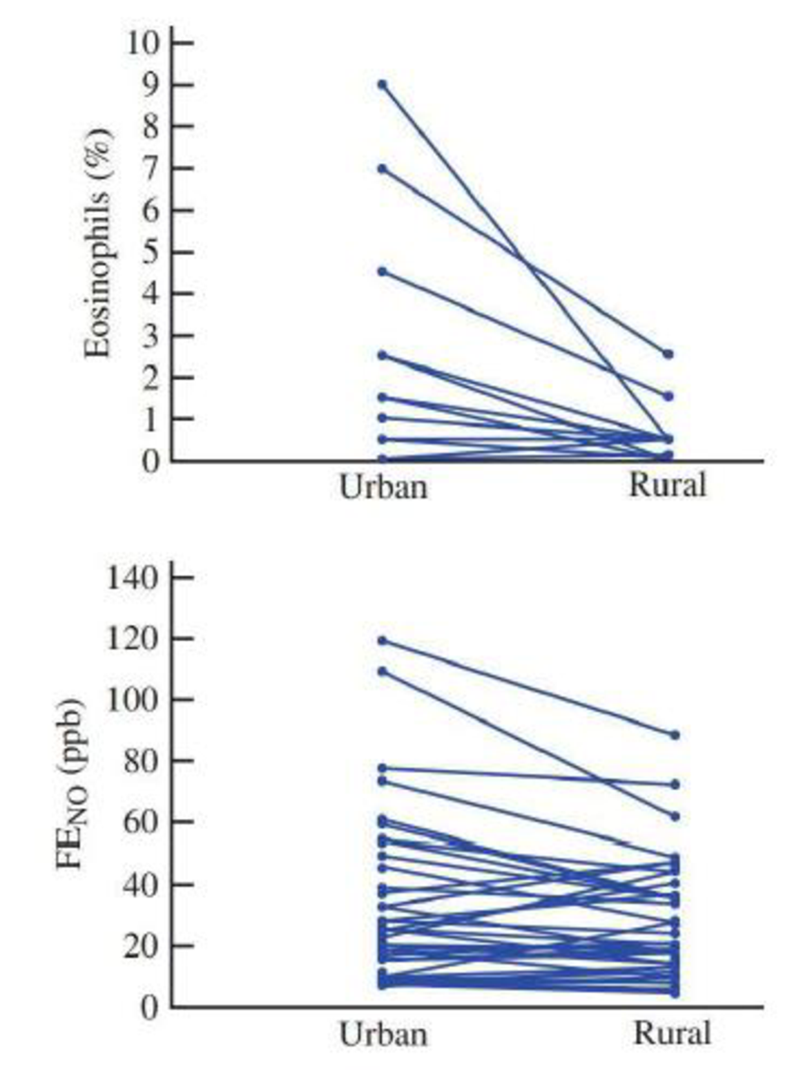
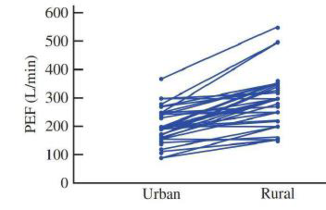
- a. Which measure (Eosinophils, FENO, or PEF) do you think resulted in a test with the P-value that was less than 0.001? Explain your reasoning.
- b. Which measure (Eosinophils, FENO, or PEF) do you think resulted in the test with the largest P-value? Explain your reasoning.
Want to see the full answer?
Check out a sample textbook solution
Chapter 11 Solutions
Introduction to Statistics and Data Analysis
- Reduced heart rate variability (HRV) is known to be a predictor of mortality after a heart attack. One measure of HRV is the average of normal-to-normal beat interval (in milliseconds) for a 24-hour time period. Twenty-two heart attack patients who were dog owners and 80 heart attack patients who did not own a dog participated in a study of the effect of pet ownership on HRV, resulting in the summary statistics shown in the accompanying table. Measure ofHRV (averagenormal-to-normalbeat interval) Mean StandardDeviation Owns Dog 874 136 Does Not Own Dog 801 133 (a) The authors of this paper used a two-sample t test to test H0: ?1 - ?2 = 0 versus Ha: ?1 - ?2 ≠ 0. What assumptions must be reasonable in order for this to be an appropriate method of analysis?We must assume that the population distributions ---Select--- are aren't approximately normal.(b) The paper indicates that the null hypothesis from Part (a) was rejected and reports that the P-value is less than…arrow_forwardBlood cocaine concentration (mg/L) was determinedboth for a sample of individuals who had died fromcocaine-induced excited delirium (ED) and for a sampleof those who had died from a cocaine overdose withoutexcited delirium; survival time for people in bothgroups was at most 6 hours. The accompanying datawas read from a comparative boxplot in the article“Fatal Excited Delirium Following Cocaine Use” (J.of Forensic Sciences, 1997: 25–31). ED 0 0 0 0 .1 .1 .1 .1 .2 .2 .3 .3.3 .4 .5 .7 .8 1.0 1.5 2.7 2.83.5 4.0 8.9 9.2 11.7 21.0Non-ED 0 0 0 0 0 .1 .1 .1 .1 .2 .2 .2.3 .3 .3 .4 .5 .5 .6 .8 .9 1.01.2 1.4 1.5 1.7 2.0 3.2 3.5 4.14.3 4.8 5.0 5.6 5.9 6.0 6.4 7.98.3 8.7 9.1 9.6 9.9 11.0 11.512.2 12.7 14.0 16.6 17.8 a. Determine the medians, fourths, and fourth spreadsfor the two samples.b. Are there any outliers in either sample? Any extremeoutliers?c. Construct a comparative boxplot, and use it as abasis for comparing and contrasting the ED andnon-ED samples.arrow_forwardAnemia (low healthy blood cells or hemoglobin) has an important role in exercise performance. However, the direct link between rapid changes of hemoglobin and exercise performance is still unknown. A study investigated 18 patients with a blood disorder (beta-thalassemia). Participants in the study performed an exercise test before and the day after receiving a blood transfusion. Data are given in the table. HB = Hemoglobin RER = Respiratory exchange ID Change in HB Obese RER > 1.1 ratio No No 1 -1.4 No -1.5 No Yes No Yes 3 -2 No 4 -2.1 No -1.9 Yes Yes No -1.6 -1.8 -0.8 6 7 No Yes No Yes 8 9. -1 No No -1.2 No Yes 10 11 No No -0.8 -1.5 12 Yes No No Yes 13 14 -1.4 -2.6 -1.7 No No Yes Yes 15 Yes No Yes Yes 16 -2.6 No 17 18 -2.7 -1.5 Noarrow_forward
- Carter et al investigated the effect of age at onset of bipolar disorder on the course of the illness. One of the variables studied was the subjects' family history. The table below shows the frequency of a family history of mood disorders in the two groups of interest: early age at onset (18years or younger) and later age at onset (later than 18 years old). Can we conclude on the basis of these data that subjects 18 or younger differ from subjects older than 18 with respect to family histories ofmood disorders? Ref: J Psychiatric Research 37(2003), 297-303.arrow_forwardEfforts by airlines to improve on-time arrival rates are showing results. Boston.com reports that in the first 10 months of 2012 on-time arrival rates at U.S. airports were the highest they have been since 2003. During this period 82% of flights landed within 15 minutes of their scheduled time. Are there differences among the major airlines? The data in Sheet 35 show the number of on-time arrivals for samples of flight taken from seven major U.S. airlines in 2012. Using a 0.05 level of significance, what is the p-value and what is your conclusion? Sheet 35 Arrivals American Airlines Continental Airlines Delta Airlines JetBlue Airlines Southwest Airlines United Airlines US Airways On-time 83 54 96 60 69 66 68 Late 16 18 21 22 23 15 12 99 72 117 82 92 81 80 Select one: a) Chi-square statistic = 4.32, p-value = 0.034, reject the null hypothesis, there is a statistically significant differences in the proportion of on-time arrivals b) Chi-square statistic = 7.370,…arrow_forwardHeight and Breast Cancer. In the article “Height and Weight at Various Ages and Risk of Breast Cancer” (Annals of Epidemiology, Vol. 2, pp. 597–609), L. Brinton and C. Swanson discussed the relationship between height and breast cancer. The study, sponsored by the National Cancer Institute, took 5 years and involved more than 1500 women with breast cancer and 2000 women without breast cancer; it revealed a trend between height and breast cancer: “. . . taller women have a 50 to 80 percent greater risk of getting breast cancer than women who are closer to 5 feet tall.” Christine Swanson, a nutritionist who was involved with the study, added, “. . . height may be associated with the culprit, . . . but no one really knows” the exact relationship between height and the risk of breast cancer. a. Classify this study as either an observational study or a designed experiment. Explain your answer. b. Interpret the statement made by Christine Swanson in light of your answer to part (a).arrow_forward
- An article in Plant Disease, "Effect of Nitrogen and Potassium Fertilizer Rates on Severity of Xanthomonas Blight of Syngonium Podophyllum" (1989, Vol. 73, No. 12, pp. 972-975) showed the effect of the variable nitrogen and potassium rates on the growth of "White Butterfly" and the mean percentage of disease. Data representative of that collected in this experiment is provided in the following table. Potassium (mg/pot/wk) Nitrogen (mg/pot/wk) 30 90 120 50 60.8 60.8 45.5 43.0 60.0 58.4 150 54.4 56.1 53.8 51.6 34.5 35.5 250 42.9 40.0 36.1 37.9 33.0 33.3 (a) Use the analysis of variance to test the appropriate hypotheses with a = 0.05. The effect of the variable nitrogen significant, the effect of the potassium rates significant, the interaction between the variable nitrogen and potassium rates significant. (b) Graphically analyze the residuals from this experiment. The residuals acceptable. (c) Estimate the appropriate variance component. Round your answers to 2 decimal places. Source…arrow_forwardSociodemographic differences in lung cancer worry. Hahn (2017) evaluated sociodemographic differences in how people worry about lung cancer. Some of the differences observed across demographic of interest were between males and females [t[45]=0.69; higher mean worry among men], smokers and nonsmokers [t[45]=2.69; higher mean worry among smokers]. However, at least one of these results were not statistically significant. Use the information provided to state which t test or t test did not reach the .05 level of significance in this study. (a) Compute the proportion of variance using omega-squared. (b) Suppose the pooled sample standard deviation for this test is 0.74. Using this value, compute estimated Cohen's d.arrow_forward10arrow_forward
- 10arrow_forwardAn experiment was conducted to evaluate the effect of decreases in frontalis muscle tension on headaches. The number of headaches experienced in a 2-week baseline period was recorded in 9 subjects who had been experiencing tension headaches. Then the subjects were trained to lower frontalis muscle tension using biofeedback, after which the number of headaches in another 2-week period was again recorded. The data are shown below. No. of Headaches Subject No Baseline After Training 1 17 3 2 13 7 3 6 2 4 5 3 5 5 6 6 10 2 7 8 1 8 6 0 9 7 2 Assume the t-test cannot be used because of an extreme violation of its normality assumption. Use the Wilcoxon signed ranks test to analyze the data. What do you conclude, using α = 0.05 2tail?arrow_forwardA diabetic person is interested in determining how the amount of aerobic exercise impacts his blood sugar. When blood sugar reaches 170 mg/dl, he goes out for a run at a pace of 10 minutes per mile. On different days, he runs different distances and measures his blood sugar after completing his run. The preferred blood sugar level is in the range of 80 to120 mg/dl. Levels that are too low or too high are extremely dangerous. The data generated are given in the following table: Distance (miles),x Blood sugar(mg/dl gram),y 2 136 2 146 2.5 131 2.5 125 3 120 3 116 3.5 104 3.5 95 4 85 4 94 4.5 83 4.5 75 Based on the scenario above, analyse the data with appropriate statistical methods and describe your findings in details. Use alpha=0.05 [note: use hypothesis, test statistics confidence interval etc.] ]arrow_forward
 Linear Algebra: A Modern IntroductionAlgebraISBN:9781285463247Author:David PoolePublisher:Cengage Learning
 Glencoe Algebra 1, Student Edition, 9780079039897...AlgebraISBN:9780079039897Author:CarterPublisher:McGraw Hill
 Big Ideas Math A Bridge To Success Algebra 1: Stu...AlgebraISBN:9781680331141Author:HOUGHTON MIFFLIN HARCOURTPublisher:Houghton Mifflin Harcourt
