Chapter 10, Problem 10.28P

To determine

The steady-state error due to a unit-ramp command and due to a unit-ramp disturbance of I controller with an internal feedback loop of first order plant for the given cases.

Answer to Problem 10.28P

The steady-state error values for all the cases are:

Case 1. For $\zeta =0.707$ ,

Error due to unit-ramp command: $e_{ss}=0.2$

Error due to unit-ramp disturbance: $e_{ss}=0.005$

Case 2. For $\zeta =1$ ,

Error due to unit-ramp command: $e_{ss}=0.4$

Error due to unit-ramp disturbance: $e_{ss}=0.01$

Case 3. For a root separation factor of 10,

Error due to unit-ramp command: $e_{ss}=0.22$

Error due to unit-ramp disturbance: $e_{ss}=0.001$.

Explanation of Solution

Given:

The I controller with an internal feedback loop of first order plant is as shown below:

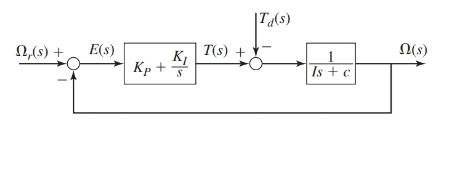
Where, the parameter values are as given:

$I=c=4$

Also, the performance specifications require the time constant of the system to be $\tau =0.2$.

The values of gains for the I controller are as follows:

Case 1. For $\zeta =0.707$, $K_I=200$ and $K_2=36$.

Case 2. For $\zeta =1$, $K_I=100$ and $K_2=36$.

Case 3. For a root separation factor of 10, $K_I=1000$ and $K_2=216$.

Concept Used:

1. The transfer functions for the block diagram are as shown below:

$\begin{array}{l}\frac{\Omega \left(s\right)}{{\Omega }_r\left(s\right)}=\frac{K_I}{I{s}^2+s\left(c+K_2\right)+K_I}\\ \frac{\Omega \left(s\right)}{T_d\left(s\right)}=\frac{-s}{I{s}^2+s\left(c+K_2\right)+K_I}\end{array}$

2. The steady-state error of a system using final value theorem is:

$e_{ss}=\underset{s\to 0}{\lim }sE\left(s\right)$.

Calculation:

From the block diagram as shown, the transfer functions are as:

$\begin{array}{l}\frac{\Omega \left(s\right)}{{\Omega }_r\left(s\right)}=\frac{K_I}{I{s}^2+s\left(c+K_2\right)+K_I}\\ \frac{\Omega \left(s\right)}{T_d\left(s\right)}=\frac{-s}{I{s}^2+s\left(c+K_2\right)+K_I}\end{array}$

Therefore, the response $\Omega \left(s\right)$ for the system is:

$\Omega \left(s\right)=\frac{K_I}{I{s}^2+s\left(c+K_2\right)+K_I}{\Omega }_r\left(s\right)-\frac{s}{I{s}^2+s\left(c+K_2\right)+K_I}{T}_d\left(s\right)$

And from the block diagram shown in figure, we have

$\begin{array}{l}E\left(s\right)=\left({\Omega }_r\left(s\right)-\Omega \left(s\right)\right)\\ \Rightarrow E\left(s\right)=\left(1-\frac{K_I}{I{s}^2+s\left(c+K_2\right)+K_I}\right){\Omega }_r\left(s\right)+\frac{s}{I{s}^2+s\left(c+K_2\right)+K_I}{T}_d\left(s\right)\\ \because \Omega \left(s\right)=\frac{K_I}{I{s}^2+s\left(c+K_2\right)+K_I}{\Omega }_r\left(s\right)-\frac{s}{I{s}^2+s\left(c+K_2\right)+K_I}{T}_d\left(s\right)\end{array}$

On keeping the values of the parameters such that $I=c=4$

$\begin{array}{l}E\left(s\right)=\left(1-\frac{K_I}{I{s}^2+s\left(c+K_2\right)+K_I}\right){\Omega }_r\left(s\right)+\frac{s}{I{s}^2+s\left(c+K_2\right)+K_I}{T}_d\left(s\right)\\ \Rightarrow E\left(s\right)=\left(\frac{s\left(Is+c+K_2\right)}{I{s}^2+s\left(c+K_2\right)+K_I}\right){\Omega }_r\left(s\right)+\frac{s}{I{s}^2+s\left(c+K_2\right)+K_I}{T}_d\left(s\right)\\ \Rightarrow E\left(s\right)=\left(\frac{s\left(4s+4+K_2\right)}{4s^2+s\left(4+K_2\right)+K_I}\right){\Omega }_r\left(s\right)+\frac{s}{4s^2+s\left(4+K_2\right)+K_I}{T}_d\left(s\right)\end{array}$

Case 1. When $\zeta =0.707$, the gain values are $K_I=200$ and $K_2=36$:

Since,

$\begin{array}{l}E\left(s\right)=\left(\frac{s\left(4s+4+K_2\right)}{4s^2+s\left(4+K_2\right)+K_I}\right){\Omega }_r\left(s\right)+\frac{s}{4s^2+s\left(4+K_2\right)+K_I}{T}_d\left(s\right)\\ \because K_I=200\text{and}{K}_2=36\\ \Rightarrow E\left(s\right)=\left(\frac{s\left(4s+4+36\right)}{4s^2+s\left(4+36\right)+200}{\Omega }_r\left(s\right)+\frac{s}{4s^2+s\left(4+36\right)+200}{T}_d\left(s\right)\right)\\ \Rightarrow E\left(s\right)=\left(\frac{s\left(4s+40\right)}{4s^2+40s+200}{\Omega }_r\left(s\right)+\frac{s}{4s^2+40s+200}{T}_d\left(s\right)\right)\end{array}$

Therefore, for unit-ramp command response ${\Omega }_r\left(s\right)$ and zero disturbance torque $T_d\left(s\right)$, we have

$\begin{array}{l}E\left(s\right)=\left(\frac{s\left(4s+40\right)}{4s^2+40s+200}{\Omega }_r\left(s\right)+\frac{s}{4s^2+40s+200}{T}_d\left(s\right)\right)\\ \Rightarrow E\left(s\right)=\left(\frac{s\left(4s+40\right)}{4s^2+40s+200}\cdot \frac{1}{s^2}+\frac{s}{4s^2+40s+200}\cdot 0\right)\\ \Rightarrow E\left(s\right)=\frac{\left(4s+40\right)}{\left(4s^2+40s+200\right)}\cdot \frac{1}{s}\\ \Rightarrow E\left(s\right)=\frac{\left(s+10\right)}{\left(s^2+10s+50\right)}\cdot \frac{1}{s}\end{array}$

Thus, the steady-state error for this design is:

$\begin{array}{l}{e}_{ss}=\underset{s\to 0}{\lim }sE\left(s\right)\\ \Rightarrow e_{ss}=\underset{s\to 0}{\lim }s\frac{\left(s+10\right)}{\left(s^2+10s+50\right)}\cdot \frac{1}{s}\because E\left(s\right)=\frac{\left(s+10\right)}{\left(s^2+10s+50\right)}\cdot \frac{1}{s}\\ \Rightarrow e_{ss}=\underset{s\to 0}{\lim }\frac{\left(s+10\right)}{\left(s^2+10s+50\right)}=\frac{10}{50}\\ \Rightarrow e_{ss}=0.2\end{array}$

Therefore, for zero command response ${\Omega }_r\left(s\right)$ and unit-ramp disturbance torque $T_d\left(s\right)$, we have

$\begin{array}{l}E\left(s\right)=\left(\frac{s\left(4s+40\right)}{4s^2+40s+200}{\Omega }_r\left(s\right)+\frac{s}{4s^2+40s+200}{T}_d\left(s\right)\right)\\ \Rightarrow E\left(s\right)=\left(\frac{s\left(4s+40\right)}{4s^2+40s+200}\cdot 0+\frac{s}{4s^2+40s+200}\cdot \frac{1}{s^2}\right)\\ \Rightarrow E\left(s\right)=\frac{1}{\left(4s^2+40s+200\right)}\cdot \frac{1}{s}\\ \Rightarrow E\left(s\right)=\frac{1}{4\left(s^2+10s+50\right)}\cdot \frac{1}{s}\end{array}$

Thus, the steady-state error for this design is:

$\begin{array}{l}{e}_{ss}=\underset{s\to 0}{\lim }sE\left(s\right)\\ \Rightarrow e_{ss}=\underset{s\to 0}{\lim }s\frac{1}{4\left(s^2+10s+50\right)}\cdot \frac{1}{s}\because E\left(s\right)=\frac{1}{4\left(s^2+10s+50\right)}\cdot \frac{1}{s}\\ \Rightarrow e_{ss}=\underset{s\to 0}{\lim }\frac{1}{4\left(s^2+10s+50\right)}=\frac{1}{200}\\ \Rightarrow e_{ss}=0.005\end{array}$

Case 2. When $\zeta =1$, the gain values are $K_I=100$ and $K_2=36$:

Since,

$\begin{array}{l}E\left(s\right)=\left(\frac{s\left(4s+4+K_2\right)}{4s^2+s\left(4+K_2\right)+K_I}\right){\Omega }_r\left(s\right)+\frac{s}{4s^2+s\left(4+K_2\right)+K_I}{T}_d\left(s\right)\\ \because K_I=100\text{and}{K}_2=36\\ \Rightarrow E\left(s\right)=\left(\frac{s\left(4s+4+36\right)}{4s^2+s\left(4+36\right)+100}{\Omega }_r\left(s\right)+\frac{s}{4s^2+s\left(4+36\right)+100}{T}_d\left(s\right)\right)\\ \Rightarrow E\left(s\right)=\left(\frac{s\left(4s+40\right)}{4s^2+40s+100}{\Omega }_r\left(s\right)+\frac{s}{4s^2+40s+100}{T}_d\left(s\right)\right)\end{array}$

Therefore, for unit-ramp command response ${\Omega }_r\left(s\right)$ and zero disturbance torque $T_d\left(s\right)$, we have

$\begin{array}{l}E\left(s\right)=\left(\frac{s\left(4s+40\right)}{4s^2+40s+100}{\Omega }_r\left(s\right)+\frac{s}{4s^2+40s+100}{T}_d\left(s\right)\right)\\ \Rightarrow E\left(s\right)=\left(\frac{s\left(4s+40\right)}{4s^2+40s+100}\cdot \frac{1}{s^2}+\frac{s}{4s^2+40s+100}\cdot 0\right)\\ \Rightarrow E\left(s\right)=\frac{\left(4s+40\right)}{\left(4s^2+40s+100\right)}\cdot \frac{1}{s}\\ \Rightarrow E\left(s\right)=\frac{\left(s+10\right)}{\left(s^2+10s+25\right)}\cdot \frac{1}{s}\end{array}$

Thus, the steady-state error for this design is:

$\begin{array}{l}{e}_{ss}=\underset{s\to 0}{\lim }sE\left(s\right)\\ \Rightarrow e_{ss}=\underset{s\to 0}{\lim }s\frac{\left(s+10\right)}{\left(s^2+10s+25\right)}\cdot \frac{1}{s}\because E\left(s\right)=\frac{\left(s+10\right)}{\left(s^2+10s+25\right)}\cdot \frac{1}{s}\\ \Rightarrow e_{ss}=\underset{s\to 0}{\lim }\frac{\left(s+10\right)}{\left(s^2+10s+25\right)}=\frac{10}{25}\\ \Rightarrow e_{ss}=0.4\end{array}$

Therefore, for zero command response ${\Omega }_r\left(s\right)$ and unit-ramp disturbance torque $T_d\left(s\right)$, we have

$\begin{array}{l}E\left(s\right)=\left(\frac{s\left(4s+40\right)}{4s^2+40s+100}{\Omega }_r\left(s\right)+\frac{s}{4s^2+40s+100}{T}_d\left(s\right)\right)\\ \Rightarrow E\left(s\right)=\left(\frac{s\left(4s+40\right)}{4s^2+40s+100}\cdot 0+\frac{s}{4s^2+40s+100}\cdot \frac{1}{s^2}\right)\\ \Rightarrow E\left(s\right)=\frac{1}{\left(4s^2+40s+100\right)}\cdot \frac{1}{s}\\ \Rightarrow E\left(s\right)=\frac{1}{4\left(s^2+10s+25\right)}\cdot \frac{1}{s}\end{array}$

Thus, the steady-state error for this design is:

$\begin{array}{l}{e}_{ss}=\underset{s\to 0}{\lim }sE\left(s\right)\\ \Rightarrow e_{ss}=\underset{s\to 0}{\lim }s\frac{1}{4\left(s^2+10s+25\right)}\cdot \frac{1}{s}\because E\left(s\right)=\frac{1}{4\left(s^2+10s+25\right)}\cdot \frac{1}{s}\\ \Rightarrow e_{ss}=\underset{s\to 0}{\lim }\frac{1}{4\left(s^2+10s+25\right)}=\frac{1}{100}\\ \Rightarrow e_{ss}=0.01\end{array}$

Case 3. For a root separation factor of 10, $K_I=1000$ and $K_2=216$.

Since,

$\begin{array}{l}E\left(s\right)=\left(\frac{s\left(4s+4+K_2\right)}{4s^2+s\left(4+K_2\right)+K_I}\right){\Omega }_r\left(s\right)+\frac{s}{4s^2+s\left(4+K_2\right)+K_I}{T}_d\left(s\right)\\ \because K_I=1000\text{and}{K}_2=216\\ \Rightarrow E\left(s\right)=\left(\frac{s\left(4s+4+216\right)}{4s^2+s\left(4+216\right)+1000}{\Omega }_r\left(s\right)+\frac{s}{4s^2+s\left(4+216\right)+1000}{T}_d\left(s\right)\right)\\ \Rightarrow E\left(s\right)=\left(\frac{s\left(4s+220\right)}{4s^2+220s+1000}{\Omega }_r\left(s\right)+\frac{s}{4s^2+220s+1000}{T}_d\left(s\right)\right)\end{array}$

Therefore, for unit-ramp command response ${\Omega }_r\left(s\right)$ and zero disturbance torque $T_d\left(s\right)$, we have

$\begin{array}{l}E\left(s\right)=\left(\frac{s\left(4s+220\right)}{4s^2+220s+1000}{\Omega }_r\left(s\right)+\frac{s}{4s^2+220s+1000}{T}_d\left(s\right)\right)\\ \Rightarrow E\left(s\right)=\left(\frac{s\left(4s+220\right)}{4s^2+220s+1000}\cdot \frac{1}{s^2}+\frac{s}{4s^2+220s+1000}\cdot 0\right)\\ \Rightarrow E\left(s\right)=\frac{\left(4s+220\right)}{\left(4s^2+220s+1000\right)}\cdot \frac{1}{s}\\ \Rightarrow E\left(s\right)=\frac{\left(s+55\right)}{\left(s^2+55s+250\right)}\cdot \frac{1}{s}\end{array}$

Thus, the steady-state error for this design is:

$\begin{array}{l}{e}_{ss}=\underset{s\to 0}{\lim }sE\left(s\right)\\ \Rightarrow e_{ss}=\underset{s\to 0}{\lim }s\frac{\left(s+55\right)}{\left(s^2+55s+250\right)}\cdot \frac{1}{s}\because E\left(s\right)=\frac{\left(s+55\right)}{\left(s^2+55s+250\right)}\cdot \frac{1}{s}\\ \Rightarrow e_{ss}=\underset{s\to 0}{\lim }\frac{\left(s+55\right)}{\left(s^2+55s+250\right)}=\frac{55}{250}\\ \Rightarrow e_{ss}=0.22\end{array}$

Therefore, for zero command response ${\Omega }_r\left(s\right)$ and unit-ramp disturbance torque $T_d\left(s\right)$, we have

$\begin{array}{l}E\left(s\right)=\left(\frac{s\left(4s+220\right)}{4s^2+220s+1000}{\Omega }_r\left(s\right)+\frac{s}{4s^2+220s+1000}{T}_d\left(s\right)\right)\\ \Rightarrow E\left(s\right)=\left(\frac{s\left(4s+220\right)}{4s^2+220s+1000}\cdot 0+\frac{s}{4s^2+220s+1000}\cdot \frac{1}{s^2}\right)\\ \Rightarrow E\left(s\right)=\frac{1}{\left(4s^2+220s+1000\right)}\cdot \frac{1}{s}\\ \Rightarrow E\left(s\right)=\frac{1}{4\left(s^2+55s+250\right)}\cdot \frac{1}{s}\end{array}$

Thus, the steady-state error for this design is:

$\begin{array}{l}{e}_{ss}=\underset{s\to 0}{\lim }sE\left(s\right)\\ \Rightarrow e_{ss}=\underset{s\to 0}{\lim }s\frac{1}{4\left(s^2+55s+250\right)}\cdot \frac{1}{s}\because E\left(s\right)=\frac{1}{4\left(s^2+55s+250\right)}\cdot \frac{1}{s}\\ \Rightarrow e_{ss}=\underset{s\to 0}{\lim }\frac{\left(s+1\right)}{4\left(s^2+55s+250\right)}=\frac{1}{1000}\\ \Rightarrow e_{ss}=0.001\end{array}$.

Conclusion:

The steady-state error values for all the cases are:

Case 1. For $\zeta =0.707$ ,

Error due to unit-ramp command: $e_{ss}=0.2$

Error due to unit-ramp disturbance: $e_{ss}=0.005$

Case 2. For $\zeta =1$, $T_m\approx 35\text{N}\cdot \text{m}$.

Error due to unit-ramp command: $e_{ss}=0.4$

Error due to unit-ramp disturbance: $e_{ss}=0.01$

Case 3. For a root separation factor of 10, $T_m\approx 215\text{N}\cdot \text{m}$.

Error due to unit-ramp command: $e_{ss}=0.22$

Error due to unit-ramp disturbance: $e_{ss}=0.001$.