Videos
i.
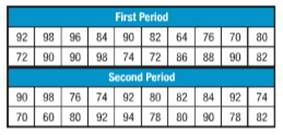
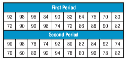
Calculate the mean, median and mode for given classes.
i.
Answer to Problem 13.1MPS
For first period,
Mean =83.7
Median = 85
Mode = 90
For second period,
Mean =82.3
Median = 81
Mode = 92
Explanation of Solution
Given:

Calculations:
Here, we have to calculate mean, median and mode for given data.
Mean is the average of given set of data.
Mean for first period is
Mean for second period is
Median is the centered value of given data.
Median for first period is
64, 70, 72, 72, 74, 76, 80, 82, 82, 84, 86, 88, 90, 90, 90, 90, 92, 96, 98, 98
Median is the centered value of given data.
Median for first period is
60, 70, 74, 74, 76, 78, 78, 80, 80, 80, 82, 82, 84, 90, 90, 92, 92, 92, 94, 98
Mode is the frequent value in given data.
Thus, in first period, 90 is mode.
In second period, 92 is mode.
Conclusion:
Therefore, we are able to find mean, median and mode of given data.
ii.
Draw stem and leaf plot for given data.
ii.
Answer to Problem 13.1MPS
Back to back stem and leaf plot for given data is
| First period | Stem | Second period |
| 4 | 6 | 0 |
| 6 4 2 2 0 | 7 | 0 4 4 6 8 8 |
| 8 6 4 2 2 0 | 8 | 0 0 0 2 2 4 |
| 8 8 6 2 0 0 0 0 | 9 | 0 0 2 2 2 4 8 |
Explanation of Solution
Given:

Calculations:
Stem and leaf plots shows the frequency of given data.
There are two parts of this plot namely stem and leaf. Stem shows first digit and leaf shows last digit.
We have given two different data. For this we has to draw back to back stem and leaf plot.
| First period | Stem | Second period |
| 4 | 6 | 0 |
| 6 4 2 2 0 | 7 | 0 4 4 6 8 8 |
| 8 6 4 2 2 0 | 8 | 0 0 0 2 2 4 |
| 8 8 6 2 0 0 0 0 | 9 | 0 0 2 2 2 4 8 |
Conclusion:
Therefore, we are able to draw back to back stem and leaf plot.
iii.
Calculate measures of variation for given data.

iii.
Answer to Problem 13.1MPS
Measures of variation for given data is,
| Measures of variation | First period | Second period |
| Range | 34 | 38 |
| Median | 75 | 81 |
| Upper Quartile | 75 | 77 |
| Lower Quartile | 90 | 91 |
| Interquartile range | 15 | 14 |
Explanation of Solution
Given:

Calculations:
Here, we have to calculate measures of variation and outlier for given set of data.
Measures of variation include range, upper quartile, lower quartile and interquartile range of given data.
Range is the difference between higher and lower data value.
Here, (Range) Firstperiod = 98-64 = 34
(Range)Secondperiod = 98-60 = 38
Median for first period is 85 and for second order is 81.
Upper quartile is the median of upper half set of data.
Here, (Upper quartile)Firstperiod is,
(Upper quartile)Secondperiod is,
Lower quartile is the median of lower half set of data.
Here, (lower quartile) Firstperiod is,
(Lower quartile)Secondperiod is,
Interquartile range is the difference between upper quartile and lower quartile.
Here, (Interquartile range) Firstperiod =90-75=15
(Interquartile range)Secondperiod =91-77=14
Conclusion:
Therefore, we are able to find measures of variation for given data.
Chapter SH Solutions
Pre-Algebra Student Edition
Additional Math Textbook Solutions
Introductory Statistics
Elementary Statistics: Picturing the World (7th Edition)
College Algebra (7th Edition)
Elementary Statistics
Calculus: Early Transcendentals (2nd Edition)


- Evaluate the following expression and show your work to support your calculations. a). 6! b). 4! 3!0! 7! c). 5!2! d). 5!2! e). n! (n - 1)!arrow_forwardAmy and Samiha have a hat that contains two playing cards, one ace and one king. They are playing a game where they randomly pick a card out of the hat four times, with replacement. Amy thinks that the probability of getting exactly two aces in four picks is equal to the probability of not getting exactly two aces in four picks. Samiha disagrees. She thinks that the probability of not getting exactly two aces is greater. The sample space of possible outcomes is listed below. A represents an ace, and K represents a king. Who is correct?arrow_forwardConsider the exponential function f(x) = 12x. Complete the sentences about the key features of the graph. The domain is all real numbers. The range is y> 0. The equation of the asymptote is y = 0 The y-intercept is 1arrow_forward
- The graph shows Alex's distance from home after biking for x hours. What is the average rate of change from -1 to 1 for the function? 4-2 о A. -2 О B. 2 О C. 1 O D. -1 ty 6 4 2 2 0 X 2 4arrow_forwardWrite 7. √49 using rational exponents. ○ A. 57 47 B. 7 O C. 47 ○ D. 74arrow_forwardCan you check If my short explantions make sense because I want to make sure that I describe this part accuratelyarrow_forward
- 9! is 362, 880. What is 10!?arrow_forwardBruce and Krista are going to buy a new furniture set for their living room. They want to buy a couch, a coffee table, and a recliner. They have narrowed it down so that they are choosing between \[4\] couches, \[5\] coffee tables, and \[9\] recliners. How many different furniture combinations are possible?arrow_forwardCan you check if my step is correct?arrow_forward
 Algebra and Trigonometry (6th Edition)AlgebraISBN:9780134463216Author:Robert F. BlitzerPublisher:PEARSON
 Contemporary Abstract AlgebraAlgebraISBN:9781305657960Author:Joseph GallianPublisher:Cengage Learning
 Linear Algebra: A Modern IntroductionAlgebraISBN:9781285463247Author:David PoolePublisher:Cengage Learning
 Algebra And Trigonometry (11th Edition)AlgebraISBN:9780135163078Author:Michael SullivanPublisher:PEARSON
 Introduction to Linear Algebra, Fifth EditionAlgebraISBN:9780980232776Author:Gilbert StrangPublisher:Wellesley-Cambridge Press
 College Algebra (Collegiate Math)AlgebraISBN:9780077836344Author:Julie Miller, Donna GerkenPublisher:McGraw-Hill Education