Chapter B.3, Problem 72E

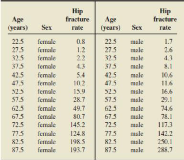
Hip Fracture Rates. Refer to Exercise B.25 on page B-25, regarding the results of a study on the rates of hip fracture for women and men in Beijing, China. In that exercise, we considered the relationship between hip fracture rate and age for women only. We now add the hip fracture rate for men to the study and consider the relationship between frac (hip fracture rate) and the predictor variable age and indicator variable sex, where

$sex=\{\begin{array}{l}1,\text{if}\text{female};\hfill \\ 0,\text{if}\text{male}.\hfill \end{array}$

Here are the data.

In Exorcise B.25 we considered transformations to straighten the scatterplot of frac versus age and investigated the regression of ln(frac) on age. Here we will regress ln(frac) on age and sex. Use the technology of your choice to do the following.

1. a. Obtain the scatterplot of ln(frac) versus age, using a different plot symbol for each sex. Based on this plot does it appear that sex is a useful predictor variable? Explain your answer.
2. b. Obtain the regression analysis of ln(frac) on age and sex. Conduct t-tests for the individual utility of the two predictor variables at the 5% level of significance. Interpret your results.
3. c. Based on the output in part (b), obtain the individual regression equations relating frac to age for females and for males.
4. d. Obtain plots of residuals versus fitted values, residuals versus age, and residuals versus sex, and a normal probability plot of the residuals. Perform a residual analysis to assess the appropriateness of the regression equation, constancy of the conditional standard deviations, and normality of the conditional distributions. Check for outliers and influential observations.
5. e. Provide a scatterplot of frac versus age with the regression curves for each sex. Based on this plot and your residual analysis in part (d), do you feel that this model fits the data well? Explain your answer.
6. f. To check for possible interaction between the two predictor variables, perform the regression analysis of ln(frac) on age, sex, and sex·age. Is there an interaction between age and sex? Use α = 0.05.