
Concept explainers
Videos
(a)
If the two sample t-procedures can be used to analyze the provided data for group differences.
(a)
Answer to Problem 71E
Solution: A t-test is appropriate to analyze the provided problem.
Explanation of Solution
Since, the population standard deviations are not known. It is replaced by sample standard deviations of the samples. Also, the sample sizes are almost equal in the provided problem, which is
(b)
The appropriate null and alternative hypotheses to compare the two groups in terms of consumption of fats.
(b)
Answer to Problem 71E
Solution: The null and alternative hypotheses are:
Explanation of Solution
Therefore, the hypotheses are formulated as:
In the above hypothesis,
(c)
To test: A significance test to determine the difference in consumption of fats in two groups.
(c)
Answer to Problem 71E
Solution: The t- test statistic is obtained as
Explanation of Solution
Calculation: To test the hypothesis formulated in part (b), the following test statistic is formulated,
Where,
The difference of means is considered as 0 according to the null hypothesis. Substitute the provided values in the above-defined formula to compute the two sample t-statistic. So,
The p-value for the provided one-sided test is calculated as
So, the degree of freedom is 199. Use Excel function to determine the exact p- value. The Excel function to determine the p- value from t-test statistic is mentioned below and the screenshot is attached,
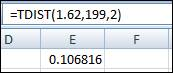
Therefore, the p-value is obtained as 0.1068.
To explain: A summary of the conclusion of the test performed above.
Answer to Problem 71E
Solution: The two groups of early eaters and late eaters have a similar average fat consumption.
Explanation of Solution
(d)
To find: A 95% confidence interval for the difference of means between early eaters and late eaters in terms of consumption of fats.
(d)
Answer to Problem 71E
Solution: The 95% confidence interval is
Explanation of Solution
Calculation: The confidence interval for the difference between the means is calculated as:
where
The t*–value for 95% confidence level is obtained as 1.97. Substitute the provided values in the above-defined formula to determine the 95% confidence interval as:
Therefore, the 95% confidence interval is obtained as
To explain: The comparison of information from obtained confidence interval with the information given by the significance test.
Answer to Problem 71E
Solution: Both the information obtained from confidence interval and the significance test shows that the null hypothesis is not rejected and concludes that there is no significant difference between the two means.
Explanation of Solution
The obtained confidence interval
Want to see more full solutions like this?
Chapter 7 Solutions
Introduction to the Practice of Statistics


- The following ordered data list shows the data speeds for cell phones used by a telephone company at an airport: A. Calculate the Measures of Central Tendency using the table in point B. B. Are there differences in the measurements obtained in A and C? Why (give at least one justified reason)? 0.8 1.4 1.8 1.9 3.2 3.6 4.5 4.5 4.6 6.2 6.5 7.7 7.9 9.9 10.2 10.3 10.9 11.1 11.1 11.6 11.8 12.0 13.1 13.5 13.7 14.1 14.2 14.7 15.0 15.1 15.5 15.8 16.0 17.5 18.2 20.2 21.1 21.5 22.2 22.4 23.1 24.5 25.7 28.5 34.6 38.5 43.0 55.6 71.3 77.8arrow_forwardIn a company with 80 employees, 60 earn $10.00 per hour and 20 earn $13.00 per hour. a) Determine the average hourly wage. b) In part a), is the same answer obtained if the 60 employees have an average wage of $10.00 per hour? Prove your answer.arrow_forwardThe following ordered data list shows the data speeds for cell phones used by a telephone company at an airport: A. Calculate the Measures of Central Tendency from the ungrouped data list. B. Group the data in an appropriate frequency table. 0.8 1.4 1.8 1.9 3.2 3.6 4.5 4.5 4.6 6.2 6.5 7.7 7.9 9.9 10.2 10.3 10.9 11.1 11.1 11.6 11.8 12.0 13.1 13.5 13.7 14.1 14.2 14.7 15.0 15.1 15.5 15.8 16.0 17.5 18.2 20.2 21.1 21.5 22.2 22.4 23.1 24.5 25.7 28.5 34.6 38.5 43.0 55.6 71.3 77.8arrow_forward
- Businessarrow_forwardhttps://www.hawkeslearning.com/Statistics/dbs2/datasets.htmlarrow_forwardNC Current Students - North Ce X | NC Canvas Login Links - North ( X Final Exam Comprehensive x Cengage Learning x WASTAT - Final Exam - STAT → C webassign.net/web/Student/Assignment-Responses/submit?dep=36055360&tags=autosave#question3659890_9 Part (b) Draw a scatter plot of the ordered pairs. N Life Expectancy Life Expectancy 80 70 600 50 40 30 20 10 Year of 1950 1970 1990 2010 Birth O Life Expectancy Part (c) 800 70 60 50 40 30 20 10 1950 1970 1990 W ALT 林 $ # 4 R J7 Year of 2010 Birth F6 4+ 80 70 60 50 40 30 20 10 Year of 1950 1970 1990 2010 Birth Life Expectancy Ox 800 70 60 50 40 30 20 10 Year of 1950 1970 1990 2010 Birth hp P.B. KA & 7 80 % 5 H A B F10 711 N M K 744 PRT SC ALT CTRLarrow_forward
- Harvard University California Institute of Technology Massachusetts Institute of Technology Stanford University Princeton University University of Cambridge University of Oxford University of California, Berkeley Imperial College London Yale University University of California, Los Angeles University of Chicago Johns Hopkins University Cornell University ETH Zurich University of Michigan University of Toronto Columbia University University of Pennsylvania Carnegie Mellon University University of Hong Kong University College London University of Washington Duke University Northwestern University University of Tokyo Georgia Institute of Technology Pohang University of Science and Technology University of California, Santa Barbara University of British Columbia University of North Carolina at Chapel Hill University of California, San Diego University of Illinois at Urbana-Champaign National University of Singapore McGill…arrow_forwardName Harvard University California Institute of Technology Massachusetts Institute of Technology Stanford University Princeton University University of Cambridge University of Oxford University of California, Berkeley Imperial College London Yale University University of California, Los Angeles University of Chicago Johns Hopkins University Cornell University ETH Zurich University of Michigan University of Toronto Columbia University University of Pennsylvania Carnegie Mellon University University of Hong Kong University College London University of Washington Duke University Northwestern University University of Tokyo Georgia Institute of Technology Pohang University of Science and Technology University of California, Santa Barbara University of British Columbia University of North Carolina at Chapel Hill University of California, San Diego University of Illinois at Urbana-Champaign National University of Singapore…arrow_forwardA company found that the daily sales revenue of its flagship product follows a normal distribution with a mean of $4500 and a standard deviation of $450. The company defines a "high-sales day" that is, any day with sales exceeding $4800. please provide a step by step on how to get the answers in excel Q: What percentage of days can the company expect to have "high-sales days" or sales greater than $4800? Q: What is the sales revenue threshold for the bottom 10% of days? (please note that 10% refers to the probability/area under bell curve towards the lower tail of bell curve) Provide answers in the yellow cellsarrow_forward
- Find the critical value for a left-tailed test using the F distribution with a 0.025, degrees of freedom in the numerator=12, and degrees of freedom in the denominator = 50. A portion of the table of critical values of the F-distribution is provided. Click the icon to view the partial table of critical values of the F-distribution. What is the critical value? (Round to two decimal places as needed.)arrow_forwardA retail store manager claims that the average daily sales of the store are $1,500. You aim to test whether the actual average daily sales differ significantly from this claimed value. You can provide your answer by inserting a text box and the answer must include: Null hypothesis, Alternative hypothesis, Show answer (output table/summary table), and Conclusion based on the P value. Showing the calculation is a must. If calculation is missing,so please provide a step by step on the answers Numerical answers in the yellow cellsarrow_forwardShow all workarrow_forward
 MATLAB: An Introduction with ApplicationsStatisticsISBN:9781119256830Author:Amos GilatPublisher:John Wiley & Sons Inc
 Probability and Statistics for Engineering and th...StatisticsISBN:9781305251809Author:Jay L. DevorePublisher:Cengage Learning
 Statistics for The Behavioral Sciences (MindTap C...StatisticsISBN:9781305504912Author:Frederick J Gravetter, Larry B. WallnauPublisher:Cengage Learning
 Elementary Statistics: Picturing the World (7th E...StatisticsISBN:9780134683416Author:Ron Larson, Betsy FarberPublisher:PEARSON
 The Basic Practice of StatisticsStatisticsISBN:9781319042578Author:David S. Moore, William I. Notz, Michael A. FlignerPublisher:W. H. Freeman
 Introduction to the Practice of StatisticsStatisticsISBN:9781319013387Author:David S. Moore, George P. McCabe, Bruce A. CraigPublisher:W. H. Freeman