
Concept explainers
Videos
Section 1:
To test: The significance test to test whether there is a difference in sprint speed of Elite players from the Canadian National team and a university squad.
Section 1:
Answer to Problem 58E
Solution: There is a significant difference between the sprint speed of both types of players. The t -statistic is 2.89 which lies between
Explanation of Solution
Calculation: The hypothesis is considered as that there is no difference in sprint speed of elite players and a university squad against the alternative that there is difference in the sprint speeds of the elite players and the university squad. Hence, the hypotheses are formulated as:
The two-sample t- test statistic is defined as:
Where,
The difference of means is considered as 0 points as the null hypothesis states that there is no difference between the two sets of players. Substitute the provided values in the above-defined formula to compute the two sample t statistic. So,
The P-value for the provided one-sided test is
So, the degree of freedom is 12. Compare the obtained value of t-statistic with the values in the table D for 12 degrees of freedom. The table D shows that the value of
To explain: The conclusion of the performed significance test.
Answer to Problem 58E
Solution: The data strongly suggests that there is a significant difference between the sprint speed of the elite players of Canadian National team and a university squad.
Explanation of Solution
Section 2:
To test: The Significance test to test whether there is difference in peak heart rate of Elite players from the Canadian National team and the university squad.
Section 2:
Answer to Problem 58E
Solution: The data strongly suggests that there is no significant difference between the peak heart rate of the elite players of Canadian National team and a university squad. The t-statistic is obtained as
Explanation of Solution
Calculation: The hypothesis is considered as that there is no difference in peak heart rate of elite players and a university squad against the alternative that there is difference in peak heart rate of the elite players and university squad. Hence, the hypotheses are formulated as:
The two-sample t- test statistic is defined as:
Where,
The difference of means is considered as 0 points as the null hypothesis states that there is no difference between the two sets of players. Substitute the provided values in the above-defined formula to compute the two sample t statistic. So,
The P-value for the provided one-sided test is
So, the degree of freedom is 12. Compare the obtained value of t- statistic with the values in the table D for 12 degrees of freedom. The table D shows that the value of
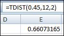
Hence, the P-value is obtained as 0.661.
To explain: The conclusion of the performed significance test.
Answer to Problem 58E
Solution: The data strongly suggests that there is no significant difference between the peak heart rate of the elite players of Canadian National team and a university squad.
Explanation of Solution
Section 3:
To test: Significance test to test whether there is difference in intermittent recovery test of Elite players from the Canadian National team and university squad.
Section 3:
Answer to Problem 58E
Solution: The data strongly suggests that there is a significant difference between the intermittent recovery test of the elite players of Canadian National team and university squad. The t- test statistic is obtained as
Explanation of Solution
Calculation: The hypothesis is considered as that there is no difference in intermittent recovery test of elite players and a university squad against the alternative that there is difference in intermittent recovery test of the elite players and university squad. Hence, the hypotheses are formulated as:
The two-sample t- test statistic is defined as:
Where
The difference of means is considered as 0 points as the null hypothesis states that there is no difference between the two sets of players. Substitute the provided values in the above-defined formula to compute the two sample t-statistic. So,
For the second approximation, the degrees of freedom k is the smaller of
So, the degree of freedom is 12. Compare the obtained value of t -statistic with the values in the table D for 12 degrees of freedom. The table D shows that the value of
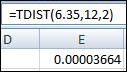
Therefore, the P-value is obtained as 0.000.
To explain: The conclusion of the performed significance test.
Answer to Problem 58E
Solution: The data strongly suggests that there is a significant difference between the intermittent recovery test of the elite players of Canadian National team and university squad.
Explanation of Solution
Want to see more full solutions like this?
Chapter 7 Solutions
Introduction to the Practice of Statistics


- Q.2.3 The probability that a randomly selected employee of Company Z is female is 0.75. The probability that an employee of the same company works in the Production department, given that the employee is female, is 0.25. What is the probability that a randomly selected employee of the company will be female and will work in the Production department? Q.2.4 There are twelve (12) teams participating in a pub quiz. What is the probability of correctly predicting the top three teams at the end of the competition, in the correct order? Give your final answer as a fraction in its simplest form.arrow_forwardQ.2.1 A bag contains 13 red and 9 green marbles. You are asked to select two (2) marbles from the bag. The first marble selected will not be placed back into the bag. Q.2.1.1 Construct a probability tree to indicate the various possible outcomes and their probabilities (as fractions). Q.2.1.2 What is the probability that the two selected marbles will be the same colour? Q.2.2 The following contingency table gives the results of a sample survey of South African male and female respondents with regard to their preferred brand of sports watch: PREFERRED BRAND OF SPORTS WATCH Samsung Apple Garmin TOTAL No. of Females 30 100 40 170 No. of Males 75 125 80 280 TOTAL 105 225 120 450 Q.2.2.1 What is the probability of randomly selecting a respondent from the sample who prefers Garmin? Q.2.2.2 What is the probability of randomly selecting a respondent from the sample who is not female? Q.2.2.3 What is the probability of randomly…arrow_forwardTest the claim that a student's pulse rate is different when taking a quiz than attending a regular class. The mean pulse rate difference is 2.7 with 10 students. Use a significance level of 0.005. Pulse rate difference(Quiz - Lecture) 2 -1 5 -8 1 20 15 -4 9 -12arrow_forward
- The following ordered data list shows the data speeds for cell phones used by a telephone company at an airport: A. Calculate the Measures of Central Tendency from the ungrouped data list. B. Group the data in an appropriate frequency table. C. Calculate the Measures of Central Tendency using the table in point B. D. Are there differences in the measurements obtained in A and C? Why (give at least one justified reason)? I leave the answers to A and B to resolve the remaining two. 0.8 1.4 1.8 1.9 3.2 3.6 4.5 4.5 4.6 6.2 6.5 7.7 7.9 9.9 10.2 10.3 10.9 11.1 11.1 11.6 11.8 12.0 13.1 13.5 13.7 14.1 14.2 14.7 15.0 15.1 15.5 15.8 16.0 17.5 18.2 20.2 21.1 21.5 22.2 22.4 23.1 24.5 25.7 28.5 34.6 38.5 43.0 55.6 71.3 77.8 A. Measures of Central Tendency We are to calculate: Mean, Median, Mode The data (already ordered) is: 0.8, 1.4, 1.8, 1.9, 3.2, 3.6, 4.5, 4.5, 4.6, 6.2, 6.5, 7.7, 7.9, 9.9, 10.2, 10.3, 10.9, 11.1, 11.1, 11.6, 11.8, 12.0, 13.1, 13.5, 13.7, 14.1, 14.2, 14.7, 15.0, 15.1, 15.5,…arrow_forwardPEER REPLY 1: Choose a classmate's Main Post. 1. Indicate a range of values for the independent variable (x) that is reasonable based on the data provided. 2. Explain what the predicted range of dependent values should be based on the range of independent values.arrow_forwardIn a company with 80 employees, 60 earn $10.00 per hour and 20 earn $13.00 per hour. Is this average hourly wage considered representative?arrow_forward
- The following is a list of questions answered correctly on an exam. Calculate the Measures of Central Tendency from the ungrouped data list. NUMBER OF QUESTIONS ANSWERED CORRECTLY ON AN APTITUDE EXAM 112 72 69 97 107 73 92 76 86 73 126 128 118 127 124 82 104 132 134 83 92 108 96 100 92 115 76 91 102 81 95 141 81 80 106 84 119 113 98 75 68 98 115 106 95 100 85 94 106 119arrow_forwardThe following ordered data list shows the data speeds for cell phones used by a telephone company at an airport: A. Calculate the Measures of Central Tendency using the table in point B. B. Are there differences in the measurements obtained in A and C? Why (give at least one justified reason)? 0.8 1.4 1.8 1.9 3.2 3.6 4.5 4.5 4.6 6.2 6.5 7.7 7.9 9.9 10.2 10.3 10.9 11.1 11.1 11.6 11.8 12.0 13.1 13.5 13.7 14.1 14.2 14.7 15.0 15.1 15.5 15.8 16.0 17.5 18.2 20.2 21.1 21.5 22.2 22.4 23.1 24.5 25.7 28.5 34.6 38.5 43.0 55.6 71.3 77.8arrow_forwardIn a company with 80 employees, 60 earn $10.00 per hour and 20 earn $13.00 per hour. a) Determine the average hourly wage. b) In part a), is the same answer obtained if the 60 employees have an average wage of $10.00 per hour? Prove your answer.arrow_forward
- The following ordered data list shows the data speeds for cell phones used by a telephone company at an airport: A. Calculate the Measures of Central Tendency from the ungrouped data list. B. Group the data in an appropriate frequency table. 0.8 1.4 1.8 1.9 3.2 3.6 4.5 4.5 4.6 6.2 6.5 7.7 7.9 9.9 10.2 10.3 10.9 11.1 11.1 11.6 11.8 12.0 13.1 13.5 13.7 14.1 14.2 14.7 15.0 15.1 15.5 15.8 16.0 17.5 18.2 20.2 21.1 21.5 22.2 22.4 23.1 24.5 25.7 28.5 34.6 38.5 43.0 55.6 71.3 77.8arrow_forwardBusinessarrow_forwardhttps://www.hawkeslearning.com/Statistics/dbs2/datasets.htmlarrow_forward
 MATLAB: An Introduction with ApplicationsStatisticsISBN:9781119256830Author:Amos GilatPublisher:John Wiley & Sons Inc
 Probability and Statistics for Engineering and th...StatisticsISBN:9781305251809Author:Jay L. DevorePublisher:Cengage Learning
 Statistics for The Behavioral Sciences (MindTap C...StatisticsISBN:9781305504912Author:Frederick J Gravetter, Larry B. WallnauPublisher:Cengage Learning
 Elementary Statistics: Picturing the World (7th E...StatisticsISBN:9780134683416Author:Ron Larson, Betsy FarberPublisher:PEARSON
 The Basic Practice of StatisticsStatisticsISBN:9781319042578Author:David S. Moore, William I. Notz, Michael A. FlignerPublisher:W. H. Freeman
 Introduction to the Practice of StatisticsStatisticsISBN:9781319013387Author:David S. Moore, George P. McCabe, Bruce A. CraigPublisher:W. H. Freeman