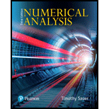
Numerical Analysis
3rd Edition
ISBN: 9780134696454
Author: Sauer, Tim
Publisher: Pearson,
expand_more
expand_more
format_list_bulleted
Textbook Question
Chapter 5.1, Problem 12E
(a) Compute the two-point forward-difference formula approximation to
explicitly, and show that it is approximately proportional to
Expert Solution & Answer
Want to see the full answer?
Check out a sample textbook solution
Students have asked these similar questions
No chatgpt pls
Remix
4. Direction Fields/Phase Portraits. Use the given direction fields to plot solution curves
to each of the given initial value problems.
(a)
x = x+2y
1111
y = -3x+y
with x(0) = 1, y(0) = -1
(b) Consider the initial value problem corresponding to the given phase portrait.
x = y
y' = 3x + 2y
Draw two "straight line solutions"
passing through (0,0)
(c) Make guesses for the equations of the straight line solutions: y = ax.
It was homework
Chapter 5 Solutions
Numerical Analysis
Ch. 5.1 - Use the two-point forward-difference formula to...Ch. 5.1 - Use the three-point centered-difference formula to...Ch. 5.1 - Use the two-point forward-difference formula to...Ch. 5.1 - Carry out the steps of Exercise 3, using the...Ch. 5.1 - Use the three-point centered-difference formula...Ch. 5.1 - Use the three-point centered-difference formula...Ch. 5.1 - Develop a formula for a two-point...Ch. 5.1 - Prove the second-order formula for the first...Ch. 5.1 - Develop a second-order formula for the first...Ch. 5.1 - Find the error term and order formula for the...
Ch. 5.1 - Find a second-order formula for approximating by...Ch. 5.1 - (a) Compute the two-point forward-difference...Ch. 5.1 - Develop a second-order method for approximating ...Ch. 5.1 - Extrapolate the formula developed in Exercise...Ch. 5.1 - Develop a first-order method for approximating ...Ch. 5.1 - Apply extrapolation to the formula developed in...Ch. 5.1 - Develop a second-order method for approximating ...Ch. 5.1 - Find, an upper bound for the error of the machine...Ch. 5.1 - Prove the second-order formula for the third...Ch. 5.1 - Prove the second-order formula for the third...Ch. 5.1 - Prob. 21ECh. 5.1 - This exercise justifies the beam equations (2.33)...Ch. 5.1 - Use Taylor expansions to prove that (5.16) is a...Ch. 5.1 - Prob. 24ECh. 5.1 - Investigate the reason for the name extrapolation....Ch. 5.1 - Make a table of the error of the three-point...Ch. 5.1 - Make a table and plot of the error of the...Ch. 5.1 - Make a table and plot of the error of the...Ch. 5.1 - Prob. 4CPCh. 5.1 - Prob. 5CPCh. 5.2 - Apply the composite Trapezoid Rule with , , and 4...Ch. 5.2 - Apply the Composite Midpoint Rule with, , and 4...Ch. 5.2 - Apply the composite Simpson’s Rule with, 2, and 4...Ch. 5.2 - Apply the composite Simpson’s Rule with, 2, and 4...Ch. 5.2 - Apply the Composite Midpoint Rule with, 2, and 4...Ch. 5.2 - Apply the Composite Midpoint Rule with, 2, and 4...Ch. 5.2 - Prob. 7ECh. 5.2 - Apply the open Newton-Cotes Rule (5.28) to...Ch. 5.2 - Apply Simpson’s Rule approximation to, and show...Ch. 5.2 - Integrate Newton’s divided-difference...Ch. 5.2 - Find the degree of precision of the following...Ch. 5.2 - Prob. 12ECh. 5.2 - Develop a composite version of the rule (5.28),...Ch. 5.2 - Prove the Composite Midpoint Rule (5.27).
Ch. 5.2 - Find the degree of precision of the degree four...Ch. 5.2 - Use the fact that the error term of Boole’s Rule...Ch. 5.2 - Prob. 17ECh. 5.2 - Prob. 1CPCh. 5.2 - Prob. 2CPCh. 5.2 - Prob. 3CPCh. 5.2 - Prob. 4CPCh. 5.2 - Prob. 5CPCh. 5.2 - Prob. 6CPCh. 5.2 - Apply the Composite Midpoint Rule to the improper...Ch. 5.2 - The arc length of the curve defined by from to ...Ch. 5.2 - Prob. 9CPCh. 5.2 - Prob. 10CPCh. 5.3 - Apply Romberg Integration to find for the...Ch. 5.3 - Apply Romberg Integration to find for the...Ch. 5.3 - Prob. 3ECh. 5.3 - Prob. 4ECh. 5.3 - Prove formula (5.31).
Ch. 5.3 - Prove formula (5.35).
Ch. 5.3 - Use Romberg Integration approximation to...Ch. 5.3 - Use Romberg Integration to approximate the...Ch. 5.3 - (a) Test the order of the second column of Romberg...Ch. 5.4 - Apply Adaptive Quadrature by hand, using the...Ch. 5.4 - Apply Adaptive Quadrature by hand, using Simpson’s...Ch. 5.4 - Prob. 3ECh. 5.4 - Develop an Adaptive Quadrature method for rule...Ch. 5.4 - Use Adaptive Trapezoid Quadrature to approximate...Ch. 5.4 - Modify the MATLAB code for Adaptive Trapezoid Rule...Ch. 5.4 - Carry out the steps of Computer Problem 1 for...Ch. 5.4 - Carry out the steps of Computer Problem 1 for the...Ch. 5.4 - Carry out the steps of Computer Problem 1 for the...Ch. 5.4 - Use Adaptive Trapezoid Quadrature to approximate...Ch. 5.4 - Carry out the steps of Problem 6, using Adaptive...Ch. 5.4 - The probability within standard deviations of the...Ch. 5.4 - Write a MATLAB function called myerf.m that uses...Ch. 5.5 - Approximate the integrals, using Gaussian...Ch. 5.5 - Prob. 2ECh. 5.5 - Approximate the integrals in Exercise 1, using ...Ch. 5.5 - Change variables, using the substitution (5.46) to...Ch. 5.5 - Approximate the integrals in Exercise 4, using ...Ch. 5.5 - Approximate the integrals, using Gaussian...Ch. 5.5 - Prob. 7ECh. 5.5 - Find the Legendre polynomials up to degree 3 and...Ch. 5.5 - Prob. 9ECh. 5.5 - Verify the coefficients and in Table 5.1 for...Ch. 5.5 - Write a MATLAB function that uses Adaptive...Ch. 5.5 - Write a program that, for any input between 0 and...Ch. 5.5 - Equipartition the path of Figure 5.6 into ...Ch. 5.5 - Prob. 4SACh. 5.5 - Prob. 5SACh. 5.5 - Prob. 6SACh. 5.5 - Write a program that traverses the path according...
Knowledge Booster
Learn more about
Need a deep-dive on the concept behind this application? Look no further. Learn more about this topic, subject and related others by exploring similar questions and additional content below.Similar questions
- No chatgpt pls will upvotearrow_forward(7) (12 points) Let F(x, y, z) = (y, x+z cos yz, y cos yz). Ꮖ (a) (4 points) Show that V x F = 0. (b) (4 points) Find a potential f for the vector field F. (c) (4 points) Let S be a surface in R3 for which the Stokes' Theorem is valid. Use Stokes' Theorem to calculate the line integral Jos F.ds; as denotes the boundary of S. Explain your answer.arrow_forward(3) (16 points) Consider z = uv, u = x+y, v=x-y. (a) (4 points) Express z in the form z = fog where g: R² R² and f: R² → R. (b) (4 points) Use the chain rule to calculate Vz = (2, 2). Show all intermediate steps otherwise no credit. (c) (4 points) Let S be the surface parametrized by T(x, y) = (x, y, ƒ (g(x, y)) (x, y) = R². Give a parametric description of the tangent plane to S at the point p = T(x, y). (d) (4 points) Calculate the second Taylor polynomial Q(x, y) (i.e. the quadratic approximation) of F = (fog) at a point (a, b). Verify that Q(x,y) F(a+x,b+y). =arrow_forward
- (6) (8 points) Change the order of integration and evaluate (z +4ry)drdy . So S√ ² 0arrow_forward(10) (16 points) Let R>0. Consider the truncated sphere S given as x² + y² + (z = √15R)² = R², z ≥0. where F(x, y, z) = −yi + xj . (a) (8 points) Consider the vector field V (x, y, z) = (▼ × F)(x, y, z) Think of S as a hot-air balloon where the vector field V is the velocity vector field measuring the hot gasses escaping through the porous surface S. The flux of V across S gives the volume flow rate of the gasses through S. Calculate this flux. Hint: Parametrize the boundary OS. Then use Stokes' Theorem. (b) (8 points) Calculate the surface area of the balloon. To calculate the surface area, do the following: Translate the balloon surface S by the vector (-15)k. The translated surface, call it S+ is part of the sphere x² + y²+z² = R². Why do S and S+ have the same area? ⚫ Calculate the area of S+. What is the natural spherical parametrization of S+?arrow_forward(1) (8 points) Let c(t) = (et, et sint, et cost). Reparametrize c as a unit speed curve starting from the point (1,0,1).arrow_forward
- (9) (16 points) Let F(x, y, z) = (x² + y − 4)i + 3xyj + (2x2 +z²)k = - = (x²+y4,3xy, 2x2 + 2²). (a) (4 points) Calculate the divergence and curl of F. (b) (6 points) Find the flux of V x F across the surface S given by x² + y²+2² = 16, z ≥ 0. (c) (6 points) Find the flux of F across the boundary of the unit cube E = [0,1] × [0,1] x [0,1].arrow_forward(8) (12 points) (a) (8 points) Let C be the circle x² + y² = 4. Let F(x, y) = (2y + e²)i + (x + sin(y²))j. Evaluate the line integral JF. F.ds. Hint: First calculate V x F. (b) (4 points) Let S be the surface r² + y² + z² = 4, z ≤0. Calculate the flux integral √(V × F) F).dS. Justify your answer.arrow_forwardDetermine whether the Law of Sines or the Law of Cosines can be used to find another measure of the triangle. a = 13, b = 15, C = 68° Law of Sines Law of Cosines Then solve the triangle. (Round your answers to four decimal places.) C = 15.7449 A = 49.9288 B = 62.0712 × Need Help? Read It Watch Itarrow_forward
- (4) (10 points) Evaluate √(x² + y² + z²)¹⁄² exp[}(x² + y² + z²)²] dV where D is the region defined by 1< x² + y²+ z² ≤4 and √√3(x² + y²) ≤ z. Note: exp(x² + y²+ 2²)²] means el (x²+ y²+=²)²]¸arrow_forward(2) (12 points) Let f(x,y) = x²e¯. (a) (4 points) Calculate Vf. (b) (4 points) Given x directional derivative 0, find the line of vectors u = D₁f(x, y) = 0. (u1, 2) such that the - (c) (4 points) Let u= (1+3√3). Show that Duƒ(1, 0) = ¦|▼ƒ(1,0)| . What is the angle between Vf(1,0) and the vector u? Explain.arrow_forwardFind the missing values by solving the parallelogram shown in the figure. (The lengths of the diagonals are given by c and d. Round your answers to two decimal places.) a b 29 39 66.50 C 17.40 d 0 54.0 126° a Ꮎ b darrow_forward
arrow_back_ios
SEE MORE QUESTIONS
arrow_forward_ios
Recommended textbooks for you
 Algebra and Trigonometry (MindTap Course List)AlgebraISBN:9781305071742Author:James Stewart, Lothar Redlin, Saleem WatsonPublisher:Cengage Learning
 College Algebra (MindTap Course List)AlgebraISBN:9781305652231Author:R. David Gustafson, Jeff HughesPublisher:Cengage Learning

 Functions and Change: A Modeling Approach to Coll...AlgebraISBN:9781337111348Author:Bruce Crauder, Benny Evans, Alan NoellPublisher:Cengage Learning
 Trigonometry (MindTap Course List)TrigonometryISBN:9781337278461Author:Ron LarsonPublisher:Cengage Learning

Algebra and Trigonometry (MindTap Course List)
Algebra
ISBN:9781305071742
Author:James Stewart, Lothar Redlin, Saleem Watson
Publisher:Cengage Learning

College Algebra (MindTap Course List)
Algebra
ISBN:9781305652231
Author:R. David Gustafson, Jeff Hughes
Publisher:Cengage Learning


Functions and Change: A Modeling Approach to Coll...
Algebra
ISBN:9781337111348
Author:Bruce Crauder, Benny Evans, Alan Noell
Publisher:Cengage Learning

Trigonometry (MindTap Course List)
Trigonometry
ISBN:9781337278461
Author:Ron Larson
Publisher:Cengage Learning
03a: Numerical Differentiation Review; Author: Jaisohn Kim;https://www.youtube.com/watch?v=IMYsqbV4CEg;License: Standard YouTube License, CC-BY