Concept explainers
Videos
(a)
To construct the
(a)
Answer to Problem 4.37E
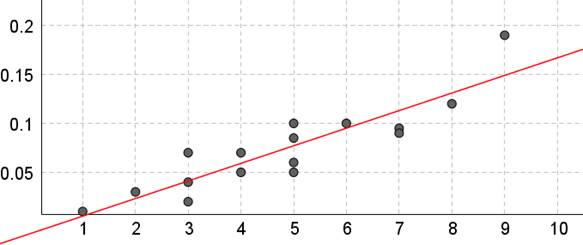
The y -variable isthe blood alcohol content.
The x -variable is the beers.
Explanation of Solution
A response variable is a variable that measures an outcome or result of a study, while an explanatory variable that we think explains or causes changes in the response variables.
The y -variable is the response variable, which we expect to be the blood alcohol content because we expect the number of beers to cause the change in the blood alcohol content.
The x -variable is the explanatory variable, which we expect to be the beers because we expect the number of beers to cause the change in the blood alcohol content.
The scatterplot of the data is as follows:
The number of beers is on the horizontal axis and the residuals are on the vertical axis.
(b)
To find the
(b)
Answer to Problem 4.37E
Explanation of Solution
Calculator commands used:
Assuming that you entered the x -values in list L1 of your calculator and the y -values in list L2 .
Use the commands STAT, CALC and 8:LinReg(
Next we determine the least square regression line by using LinReg(
The result should then contain r and r2 .
The result will be
The correlation is an appropriate measure of strength because the scatterplot in part(a) does not show strong curvature.
(c)
To find the least square regression line for BAC on beers and interpret the slope and y -intercept of the regression line.
(c)
Answer to Problem 4.37E
Explanation of Solution
Calculator commands used:
Assuming that you entered the x -values in list L1 of your calculator and the y -values in list L2 .
Use the commands STAT, CALC and 8:LinReg(
Next we determine the least square regression line by using LinReg(
Result:
Thus the least square regression line is then:
a is the y -intercept which is the predicted y -value when
b is the slope which is the average increase in the y -value per unit of
Chapter 4 Solutions
Statistics Through Applications
Additional Math Textbook Solutions
Elementary Statistics: Picturing the World (7th Edition)
Elementary Statistics
Thinking Mathematically (6th Edition)
A First Course in Probability (10th Edition)
Calculus: Early Transcendentals (2nd Edition)


- Problem 3. Pricing a multi-stock option the Margrabe formula The purpose of this problem is to price a swap option in a 2-stock model, similarly as what we did in the example in the lectures. We consider a two-dimensional Brownian motion given by W₁ = (W(¹), W(2)) on a probability space (Q, F,P). Two stock prices are modeled by the following equations: dX = dY₁ = X₁ (rdt+ rdt+0₁dW!) (²)), Y₁ (rdt+dW+0zdW!"), with Xo xo and Yo =yo. This corresponds to the multi-stock model studied in class, but with notation (X+, Y₁) instead of (S(1), S(2)). Given the model above, the measure P is already the risk-neutral measure (Both stocks have rate of return r). We write σ = 0₁+0%. We consider a swap option, which gives you the right, at time T, to exchange one share of X for one share of Y. That is, the option has payoff F=(Yr-XT). (a) We first assume that r = 0 (for questions (a)-(f)). Write an explicit expression for the process Xt. Reminder before proceeding to question (b): Girsanov's theorem…arrow_forwardProblem 1. Multi-stock model We consider a 2-stock model similar to the one studied in class. Namely, we consider = S(1) S(2) = S(¹) exp (σ1B(1) + (M1 - 0/1 ) S(²) exp (02B(2) + (H₂- M2 where (B(¹) ) +20 and (B(2) ) +≥o are two Brownian motions, with t≥0 Cov (B(¹), B(2)) = p min{t, s}. " The purpose of this problem is to prove that there indeed exists a 2-dimensional Brownian motion (W+)+20 (W(1), W(2))+20 such that = S(1) S(2) = = S(¹) exp (011W(¹) + (μ₁ - 01/1) t) 롱) S(²) exp (021W (1) + 022W(2) + (112 - 03/01/12) t). where σ11, 21, 22 are constants to be determined (as functions of σ1, σ2, p). Hint: The constants will follow the formulas developed in the lectures. (a) To show existence of (Ŵ+), first write the expression for both W. (¹) and W (2) functions of (B(1), B(²)). as (b) Using the formulas obtained in (a), show that the process (WA) is actually a 2- dimensional standard Brownian motion (i.e. show that each component is normal, with mean 0, variance t, and that their…arrow_forwardThe scores of 8 students on the midterm exam and final exam were as follows. Student Midterm Final Anderson 98 89 Bailey 88 74 Cruz 87 97 DeSana 85 79 Erickson 85 94 Francis 83 71 Gray 74 98 Harris 70 91 Find the value of the (Spearman's) rank correlation coefficient test statistic that would be used to test the claim of no correlation between midterm score and final exam score. Round your answer to 3 places after the decimal point, if necessary. Test statistic: rs =arrow_forward
- Business discussarrow_forwardBusiness discussarrow_forwardI just need to know why this is wrong below: What is the test statistic W? W=5 (incorrect) and What is the p-value of this test? (p-value < 0.001-- incorrect) Use the Wilcoxon signed rank test to test the hypothesis that the median number of pages in the statistics books in the library from which the sample was taken is 400. A sample of 12 statistics books have the following numbers of pages pages 127 217 486 132 397 297 396 327 292 256 358 272 What is the sum of the negative ranks (W-)? 75 What is the sum of the positive ranks (W+)? 5What type of test is this? two tailedWhat is the test statistic W? 5 These are the critical values for a 1-tailed Wilcoxon Signed Rank test for n=12 Alpha Level 0.001 0.005 0.01 0.025 0.05 0.1 0.2 Critical Value 75 70 68 64 60 56 50 What is the p-value for this test? p-value < 0.001arrow_forward
- ons 12. A sociologist hypothesizes that the crime rate is higher in areas with higher poverty rate and lower median income. She col- lects data on the crime rate (crimes per 100,000 residents), the poverty rate (in %), and the median income (in $1,000s) from 41 New England cities. A portion of the regression results is shown in the following table. Standard Coefficients error t stat p-value Intercept -301.62 549.71 -0.55 0.5864 Poverty 53.16 14.22 3.74 0.0006 Income 4.95 8.26 0.60 0.5526 a. b. Are the signs as expected on the slope coefficients? Predict the crime rate in an area with a poverty rate of 20% and a median income of $50,000. 3. Using data from 50 workarrow_forward2. The owner of several used-car dealerships believes that the selling price of a used car can best be predicted using the car's age. He uses data on the recent selling price (in $) and age of 20 used sedans to estimate Price = Po + B₁Age + ε. A portion of the regression results is shown in the accompanying table. Standard Coefficients Intercept 21187.94 Error 733.42 t Stat p-value 28.89 1.56E-16 Age -1208.25 128.95 -9.37 2.41E-08 a. What is the estimate for B₁? Interpret this value. b. What is the sample regression equation? C. Predict the selling price of a 5-year-old sedan.arrow_forwardian income of $50,000. erty rate of 13. Using data from 50 workers, a researcher estimates Wage = Bo+B,Education + B₂Experience + B3Age+e, where Wage is the hourly wage rate and Education, Experience, and Age are the years of higher education, the years of experience, and the age of the worker, respectively. A portion of the regression results is shown in the following table. ni ogolloo bash 1 Standard Coefficients error t stat p-value Intercept 7.87 4.09 1.93 0.0603 Education 1.44 0.34 4.24 0.0001 Experience 0.45 0.14 3.16 0.0028 Age -0.01 0.08 -0.14 0.8920 a. Interpret the estimated coefficients for Education and Experience. b. Predict the hourly wage rate for a 30-year-old worker with four years of higher education and three years of experience.arrow_forward
- 1. If a firm spends more on advertising, is it likely to increase sales? Data on annual sales (in $100,000s) and advertising expenditures (in $10,000s) were collected for 20 firms in order to estimate the model Sales = Po + B₁Advertising + ε. A portion of the regression results is shown in the accompanying table. Intercept Advertising Standard Coefficients Error t Stat p-value -7.42 1.46 -5.09 7.66E-05 0.42 0.05 8.70 7.26E-08 a. Interpret the estimated slope coefficient. b. What is the sample regression equation? C. Predict the sales for a firm that spends $500,000 annually on advertising.arrow_forwardCan you help me solve problem 38 with steps im stuck.arrow_forwardHow do the samples hold up to the efficiency test? What percentages of the samples pass or fail the test? What would be the likelihood of having the following specific number of efficiency test failures in the next 300 processors tested? 1 failures, 5 failures, 10 failures and 20 failures.arrow_forward
 MATLAB: An Introduction with ApplicationsStatisticsISBN:9781119256830Author:Amos GilatPublisher:John Wiley & Sons Inc
 Probability and Statistics for Engineering and th...StatisticsISBN:9781305251809Author:Jay L. DevorePublisher:Cengage Learning
 Statistics for The Behavioral Sciences (MindTap C...StatisticsISBN:9781305504912Author:Frederick J Gravetter, Larry B. WallnauPublisher:Cengage Learning
 Elementary Statistics: Picturing the World (7th E...StatisticsISBN:9780134683416Author:Ron Larson, Betsy FarberPublisher:PEARSON
 The Basic Practice of StatisticsStatisticsISBN:9781319042578Author:David S. Moore, William I. Notz, Michael A. FlignerPublisher:W. H. Freeman
 Introduction to the Practice of StatisticsStatisticsISBN:9781319013387Author:David S. Moore, George P. McCabe, Bruce A. CraigPublisher:W. H. Freeman