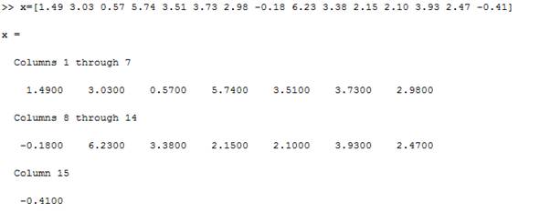
The following data, collected by U.S. Bureau of Economic Analysis, lists the year-over-year percent change in mean disposable personal income in the United States during 15 election years. Also, the proportion of the U.S. electorate that voted for the incumbent party’s presidential candidate is listed. The first line of the table says that income increased by
1.49% from 1951 to 1952, and that 44.6% of the electorate voted for Adlai Stevenson, the incumbent Democratic party’s candidate for president. Find the best least squares linear model for incumbent party vote as a function of income change. Plot this line along with the 15 data points. How many percentage points of vote can the incumbent party expect for each additional percent of change in personal income?


Want to see the full answer?
Check out a sample textbook solution
Chapter 4 Solutions
Numerical Analysis
- not use ai pleasearrow_forward4 In the integral dxf1dy (7)², make the change of variables x = ½(r− s), y = ½(r + s), and evaluate the integral. Hint: Find the limits on r and s by sketching the area of integration in the (x, y) plane along with the r and s axes, and then show that the same area can be covered by s from 0 to r and r from 0 to 1.arrow_forward7. What are all values of 0, for 0≤0<2л, where 2 sin² 0=-sin? - 5π 6 π (A) 0, л, and 6 7π (B) 0,л, 11π , and 6 6 π 3π π (C) 5π 2 2 3 , and π 3π 2π (D) 2' 2'3 , and 3 4元 3 1 די } I -2m 3 1 -3 บ 1 # 1 I 3# 3m 8. The graph of g is shown above. Which of the following is an expression for g(x)? (A) 1+ tan(x) (B) 1-tan (x) (C) 1-tan (2x) (D) 1-tan + X - 9. The function j is given by j(x)=2(sin x)(cos x)-cos x. Solve j(x) = 0 for values of x in the interval Quiz A: Topic 3.10 Trigonometric Equations and Inequalities Created by Bryan Passwaterarrow_forward
- not use ai pleasearrow_forward-xx0. B2 If Xfx(x) find the MGF in the case that fx(x) = - 1 28 exp{-|x − a\/ẞ}, Use the MGF to compute E(X) and Var(X).arrow_forwardName Assume there is the following simplified grade book: Homework Labs | Final Exam | Project Avery 95 98 90 100 Blake 90 96 Carlos 83 79 Dax 55 30 228 92 95 79 90 65 60 Assume that the weights used to compute the final grades are homework 0.3, labs 0.2, the final 0.35, and the project 0.15. | Write an explicit formula to compute Avery's final grade using a single inner product. Write an explicit formula to compute everyone's final grade simultane- ously using a single matrix-vector product.arrow_forward
- 1. Explicitly compute by hand (with work shown) the following Frobenius inner products 00 4.56 3.12 (a) ((º º º). (156 (b) 10.9 -1 0 2)), Fro 5')) Froarrow_forward3. Let 4 0 0 00 0 0 1.2 0 00 0 0 0 -10.1 0 0 0 D = 0 0 0 00 0 0 0 0 05 0 0 0 0 0 0 2.8 Either explicitly compute D-¹ or explain why it doesn't exist.arrow_forward4. [9 points] Assume that B, C, E are all 3 x 3 matrices such that BC == -64 -1 0 3 4 4 4 -2 2 CB=-1-2 4 BE -2 1 3 EC = 1 3 2 -7, 1 6 -6 2-5 -7 -2 Explicitly compute the following by hand. (I.e., write out the entries of the 3 × 3 matrix.) (a) [3 points] B(E+C) (b) [3 points] (E+B)C (c) [3 points] ETBTarrow_forward
 Glencoe Algebra 1, Student Edition, 9780079039897...AlgebraISBN:9780079039897Author:CarterPublisher:McGraw Hill
 Big Ideas Math A Bridge To Success Algebra 1: Stu...AlgebraISBN:9781680331141Author:HOUGHTON MIFFLIN HARCOURTPublisher:Houghton Mifflin Harcourt

