Chapter 4, Problem 34E

(a)

To determine

To Explain: the median or the mean for the centre of this distribution.

Explanation of Solution

Given:

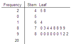
79, 80, 80, 80, 74, 80, 80, 79, 64, 78, 73, 78, 74, 45, 81, 48, 80, 82, 82, 70

Stem plot

Stem unit = 10

Leaf unit = 1

  

Median and IQR

The data is shows that the skewed left and although median and IQR are unbiased indicators and are not affected by the skewed of the distribution, they are more accurate measures in this case.

(b)

To determine

To find: the median.

Answer to Problem 34E

Explanation of Solution

Given:

79, 80, 80, 80, 74, 80, 80, 79, 64, 78, 73, 78, 74, 45, 81, 48, 80, 82, 82, 70

There are total number of values is 20 therefore the median would be average of 10^th and 11^th value of given ordered data list. 10^th and 11^th values are 79 games and 79 game respectively there the median is 79 games.

(c)

To determine

To find: that the mean is higher or lower than the median without finding the mean.

Answer to Problem 34E

Lower

Explanation of Solution

Given:

79, 80, 80, 80, 74, 80, 80, 79, 64, 78, 73, 78, 74, 45, 81, 48, 80, 82, 82, 70

Lower

Because the distribution has a longer left tail, it would expect the left tail, and therefore the lower values, to pull the overall mean down.