Concept explainers
Videos
(a)
To construct: the stem plot on the basis of given data.
(a)
Explanation of Solution
Given:
79, 80, 80, 80, 74, 80, 80, 79, 64, 78, 73, 78, 74, 45, 81, 48, 80, 82, 82, 70
Graph:
Stem plot
Stem unit = 10
Leaf unit = 1
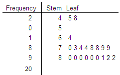
By seeing the distribution, it is observed that the shape is skewed to the left where there are more numbers on the right than on the left.
(b)
To Explain: the shape of the distribution.
(b)
Answer to Problem 32E
Skewed to the left
Explanation of Solution
The shape of the distribution is skewed to the left although there are more numbers on the right than on the left (i.e., there is a tail on the left).
(c)
To Explain: the centre and spread of the given distribution.
(c)
Explanation of Solution
The centre is at 79 if there are using the
(d)
To find: the unusual feature.
(d)
Explanation of Solution
All but three number of season are less than 70. Only one number is in the 60s and no numbers are in the 50s. The numbers 45 and 48 are very likely to be outliers. He might have injuries in these seasons that caused him to play fewer games than usual.
Chapter 4 Solutions
Stats: Modeling the World Nasta Edition Grades 9-12
Additional Math Textbook Solutions
University Calculus: Early Transcendentals (4th Edition)
Calculus: Early Transcendentals (2nd Edition)
Elementary Statistics
Introductory Statistics
Elementary Statistics: Picturing the World (7th Edition)
Intro Stats, Books a la Carte Edition (5th Edition)


- Suppose a sample of O-rings was obtained and the wall thickness (in inches) of each was recorded. Use a normal probability plot to assess whether the sample data could have come from a population that is normally distributed. Click here to view the table of critical values for normal probability plots. Click here to view page 1 of the standard normal distribution table. Click here to view page 2 of the standard normal distribution table. 0.191 0.186 0.201 0.2005 0.203 0.210 0.234 0.248 0.260 0.273 0.281 0.290 0.305 0.310 0.308 0.311 Using the correlation coefficient of the normal probability plot, is it reasonable to conclude that the population is normally distributed? Select the correct choice below and fill in the answer boxes within your choice. (Round to three decimal places as needed.) ○ A. Yes. The correlation between the expected z-scores and the observed data, , exceeds the critical value, . Therefore, it is reasonable to conclude that the data come from a normal population. ○…arrow_forwardding question ypothesis at a=0.01 and at a = 37. Consider the following hypotheses: 20 Ho: μ=12 HA: μ12 Find the p-value for this hypothesis test based on the following sample information. a. x=11; s= 3.2; n = 36 b. x = 13; s=3.2; n = 36 C. c. d. x = 11; s= 2.8; n=36 x = 11; s= 2.8; n = 49arrow_forward13. A pharmaceutical company has developed a new drug for depression. There is a concern, however, that the drug also raises the blood pressure of its users. A researcher wants to conduct a test to validate this claim. Would the manager of the pharmaceutical company be more concerned about a Type I error or a Type II error? Explain.arrow_forward
- Find the z score that corresponds to the given area 30% below z.arrow_forwardFind the following probability P(z<-.24)arrow_forward3. Explain why the following statements are not correct. a. "With my methodological approach, I can reduce the Type I error with the given sample information without changing the Type II error." b. "I have already decided how much of the Type I error I am going to allow. A bigger sample will not change either the Type I or Type II error." C. "I can reduce the Type II error by making it difficult to reject the null hypothesis." d. "By making it easy to reject the null hypothesis, I am reducing the Type I error."arrow_forward
- Given the following sample data values: 7, 12, 15, 9, 15, 13, 12, 10, 18,12 Find the following: a) Σ x= b) x² = c) x = n d) Median = e) Midrange x = (Enter a whole number) (Enter a whole number) (use one decimal place accuracy) (use one decimal place accuracy) (use one decimal place accuracy) f) the range= g) the variance, s² (Enter a whole number) f) Standard Deviation, s = (use one decimal place accuracy) Use the formula s² ·Σx² -(x)² n(n-1) nΣ x²-(x)² 2 Use the formula s = n(n-1) (use one decimal place accuracy)arrow_forwardTable of hours of television watched per week: 11 15 24 34 36 22 20 30 12 32 24 36 42 36 42 26 37 39 48 35 26 29 27 81276 40 54 47 KARKE 31 35 42 75 35 46 36 42 65 28 54 65 28 23 28 23669 34 43 35 36 16 19 19 28212 Using the data above, construct a frequency table according the following classes: Number of Hours Frequency Relative Frequency 10-19 20-29 |30-39 40-49 50-59 60-69 70-79 80-89 From the frequency table above, find a) the lower class limits b) the upper class limits c) the class width d) the class boundaries Statistics 300 Frequency Tables and Pictures of Data, page 2 Using your frequency table, construct a frequency and a relative frequency histogram labeling both axes.arrow_forwardTable of hours of television watched per week: 11 15 24 34 36 22 20 30 12 32 24 36 42 36 42 26 37 39 48 35 26 29 27 81276 40 54 47 KARKE 31 35 42 75 35 46 36 42 65 28 54 65 28 23 28 23669 34 43 35 36 16 19 19 28212 Using the data above, construct a frequency table according the following classes: Number of Hours Frequency Relative Frequency 10-19 20-29 |30-39 40-49 50-59 60-69 70-79 80-89 From the frequency table above, find a) the lower class limits b) the upper class limits c) the class width d) the class boundaries Statistics 300 Frequency Tables and Pictures of Data, page 2 Using your frequency table, construct a frequency and a relative frequency histogram labeling both axes.arrow_forward
- A study was undertaken to compare respiratory responses of hypnotized and unhypnotized subjects. The following data represent total ventilation measured in liters of air per minute per square meter of body area for two independent (and randomly chosen) samples. Analyze these data using the appropriate non-parametric hypothesis test. Unhypnotized: 5.0 5.3 5.3 5.4 5.9 6.2 6.6 6.7 Hypnotized: 5.8 5.9 6.2 6.6 6.7 6.1 7.3 7.4arrow_forwardThe class will include a data exercise where students will be introduced to publicly available data sources. Students will gain experience in manipulating data from the web and applying it to understanding the economic and demographic conditions of regions in the U.S. Regions and topics of focus will be determined (by the student with instructor approval) prior to April. What data exercise can I do to fulfill this requirement? Please explain.arrow_forwardConsider the ceocomp dataset of compensation information for the CEO’s of 100 U.S. companies. We wish to fit aregression model to assess the relationship between CEO compensation in thousands of dollars (includes salary andbonus, but not stock gains) and the following variates:AGE: The CEOs age, in yearsEDUCATN: The CEO’s education level (1 = no college degree; 2 = college/undergrad. degree; 3 = grad. degree)BACKGRD: Background type(1= banking/financial; 2 = sales/marketing; 3 = technical; 4 = legal; 5 = other)TENURE: Number of years employed by the firmEXPER: Number of years as the firm CEOSALES: Sales revenues, in millions of dollarsVAL: Market value of the CEO's stock, in natural logarithm unitsPCNTOWN: Percentage of firm's market value owned by the CEOPROF: Profits of the firm, before taxes, in millions of dollars1) Create a scatterplot matrix for this dataset. Briefly comment on the observed relationships between compensationand the other variates.Note that companies with negative…arrow_forward
 MATLAB: An Introduction with ApplicationsStatisticsISBN:9781119256830Author:Amos GilatPublisher:John Wiley & Sons Inc
 Probability and Statistics for Engineering and th...StatisticsISBN:9781305251809Author:Jay L. DevorePublisher:Cengage Learning
 Statistics for The Behavioral Sciences (MindTap C...StatisticsISBN:9781305504912Author:Frederick J Gravetter, Larry B. WallnauPublisher:Cengage Learning
 Elementary Statistics: Picturing the World (7th E...StatisticsISBN:9780134683416Author:Ron Larson, Betsy FarberPublisher:PEARSON
 The Basic Practice of StatisticsStatisticsISBN:9781319042578Author:David S. Moore, William I. Notz, Michael A. FlignerPublisher:W. H. Freeman
 Introduction to the Practice of StatisticsStatisticsISBN:9781319013387Author:David S. Moore, George P. McCabe, Bruce A. CraigPublisher:W. H. Freeman