Videos
Obtaining exact, or approximate, expressions for eigenvalues and eigenvectors in terms of the model parameters is often useful for understanding the qualitative behavior of solutions to a dynamical system. We illustrate using Example
(a) Show that the general solution of Eqs.
where
(b) Assuming that
(c) Show that approximations to the corresponding eigenvectors are
(d) Use the approximations obtained in parts (b) and (c) and the equilibrium solution
(e) Show that when
where
(f) Give a physical explanation of the significance of the eigenvalues on the dynamical behavior of the solution
Example
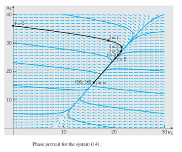
Consider the schematic diagram of the greenhouse/rockbed system in Figure
Rocks are a good material for storing heat since they have a high energy-storage capacity, are inexpensive, and have a long life.
Using
Section
Find the equilibrium solution, or critical point, of Eqs.
In the limiting case,
Thus, if initial conditions
Want to see the full answer?
Check out a sample textbook solution
Chapter 3 Solutions
Differential Equations: An Introduction to Modern Methods and Applications
Additional Math Textbook Solutions
Basic Business Statistics, Student Value Edition
Thinking Mathematically (6th Edition)
College Algebra with Modeling & Visualization (5th Edition)
A First Course in Probability (10th Edition)
Precalculus: Mathematics for Calculus (Standalone Book)
Elementary Statistics: Picturing the World (7th Edition)


- 10) Find n(K) given that n(T) = 7,n(KT) = 5,n(KUT) = 13.arrow_forward7) Use the Venn Diagram below to determine the sets A, B, and U. A = B = U = Blue Orange white Yellow Black Pink Purple green Grey brown Uarrow_forward8. For x>_1, the continuous function g is decreasing and positive. A portion of the graph of g is shown above. For n>_1, the nth term of the series summation from n=1 to infinity a_n is defined by a_n=g(n). If intergral 1 to infinity g(x)dx converges to 8, which of the following could be true? A) summation n=1 to infinity a_n = 6. B) summation n=1 to infinity a_n =8. C) summation n=1 to infinity a_n = 10. D) summation n=1 to infinity a_n diverges.arrow_forward
- 1) Use the roster method to list the elements of the set consisting of: a) All positive multiples of 3 that are less than 20. b) Nothing (An empty set).arrow_forward2) Let M = {all postive integers), N = {0,1,2,3... 100), 0= {100,200,300,400,500). Determine if the following statements are true or false and explain your reasoning. a) NCM b) 0 C M c) O and N have at least one element in common d) O≤ N e) o≤o 1arrow_forward4) Which of the following universal sets has W = {12,79, 44, 18) as a subset? Choose one. a) T = {12,9,76,333, 44, 99, 1000, 2} b) V = {44,76, 12, 99, 18,900,79,2} c) Y = {76,90, 800, 44, 99, 55, 22} d) x = {79,66,71, 4, 18, 22,99,2}arrow_forward
- 3) What is the universal set that contains all possible integers from 1 to 8 inclusive? Choose one. a) A = {1, 1.5, 2, 2.5, 3, 3.5, 4, 4.5, 5, 5.5, 6, 6.5, 7, 7.5, 8} b) B={-1,0,1,2,3,4,5,6,7,8} c) C={1,2,3,4,5,6,7,8} d) D = {0,1,2,3,4,5,6,7,8}arrow_forwardA smallish urn contains 25 small plastic bunnies – 7 of which are pink and 18 of which are white. 10 bunnies are drawn from the urn at random with replacement, and X is the number of pink bunnies that are drawn. (a) P(X = 5) ≈ (b) P(X<6) ≈ The Whoville small urn contains 100 marbles – 60 blue and 40 orange. The Grinch sneaks in one night and grabs a simple random sample (without replacement) of 15 marbles. (a) The probability that the Grinch gets exactly 6 blue marbles is [ Select ] ["≈ 0.054", "≈ 0.043", "≈ 0.061"] . (b) The probability that the Grinch gets at least 7 blue marbles is [ Select ] ["≈ 0.922", "≈ 0.905", "≈ 0.893"] . (c) The probability that the Grinch gets between 8 and 12 blue marbles (inclusive) is [ Select ] ["≈ 0.801", "≈ 0.760", "≈ 0.786"] . The Whoville small urn contains 100 marbles – 60 blue and 40 orange. The Grinch sneaks in one night and grabs a simple random sample (without replacement) of 15 marbles. (a)…arrow_forwardUsing Karnaugh maps and Gray coding, reduce the following circuit represented as a table and write the final circuit in simplest form (first in terms of number of gates then in terms of fan-in of those gates).arrow_forward
 Algebra & Trigonometry with Analytic GeometryAlgebraISBN:9781133382119Author:SwokowskiPublisher:Cengage