Students’ Ages Here are the ages of some students in a statistics class: 17, 19, 35, 18, 18, 20, 27, 25, 41, 21, 19, 19, 45, and 19. The teacher’s age is 66 and should be included as one of the ages when you do the calculations. The figure shows a histogram of the data. a. Describe the distribution of ages by giving the shape, the numerical value for an appropriate measure of the center, and the numerical value for an appropriate measure of spread, as well as mentioning any outliers. b. Make a rough sketch (or copy) of the histogram, and mark the approximate locations of the mean and of the median . Why are they not at the same location?
Students’ Ages Here are the ages of some students in a statistics class: 17, 19, 35, 18, 18, 20, 27, 25, 41, 21, 19, 19, 45, and 19. The teacher’s age is 66 and should be included as one of the ages when you do the calculations. The figure shows a histogram of the data. a. Describe the distribution of ages by giving the shape, the numerical value for an appropriate measure of the center, and the numerical value for an appropriate measure of spread, as well as mentioning any outliers. b. Make a rough sketch (or copy) of the histogram, and mark the approximate locations of the mean and of the median . Why are they not at the same location?
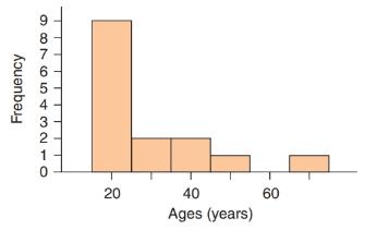
Students’ Ages Here are the ages of some students in a statistics class: 17, 19, 35, 18, 18, 20, 27, 25, 41, 21, 19, 19, 45, and 19. The teacher’s age is 66 and should be included as one of the ages when you do the calculations. The figure shows a histogram of the data.
a. Describe the distribution of ages by giving the shape, the numerical value for an appropriate measure of the center, and the numerical value for an appropriate measure of spread, as well as mentioning any outliers.
b. Make a rough sketch (or copy) of the histogram, and mark the approximate locations of the mean and of the median. Why are they not at the same location?
Statistics that help describe, summarize, and present information extracted from data. Descriptive statistics include concepts related to measures of central tendency, measures of variability, measures of frequency, shape of distribution, and some data visualization techniques/tools such as pivot tables, charts, and graphs.
2 (VaR and ES) Suppose X1
are independent. Prove that
~
Unif[-0.5, 0.5] and X2
VaRa (X1X2) < VaRa(X1) + VaRa (X2).
~
Unif[-0.5, 0.5]
8 (Correlation and Diversification)
Assume we have two stocks, A and B, show that a particular combination
of the two stocks produce a risk-free portfolio when the correlation between
the return of A and B is -1.
9 (Portfolio allocation)
Suppose R₁ and R2 are returns of 2 assets and with expected return and
variance respectively r₁ and 72 and variance-covariance σ2, 0%½ and σ12. Find
−∞ ≤ w ≤ ∞ such that the portfolio wR₁ + (1 - w) R₂ has the smallest
risk.
Need a deep-dive on the concept behind this application? Look no further. Learn more about this topic, statistics and related others by exploring similar questions and additional content below.


 Glencoe Algebra 1, Student Edition, 9780079039897...AlgebraISBN:9780079039897Author:CarterPublisher:McGraw Hill
 Holt Mcdougal Larson Pre-algebra: Student Edition...AlgebraISBN:9780547587776Author:HOLT MCDOUGALPublisher:HOLT MCDOUGAL
 Big Ideas Math A Bridge To Success Algebra 1: Stu...AlgebraISBN:9781680331141Author:HOUGHTON MIFFLIN HARCOURTPublisher:Houghton Mifflin Harcourt