Introductory Statistics (2nd Edition)
2nd Edition
ISBN: 9780321978271
Author: Robert Gould, Colleen N. Ryan
Publisher: PEARSON
expand_more
expand_more
format_list_bulleted
Concept explainers
Videos
Textbook Question
Chapter 3, Problem 57SE
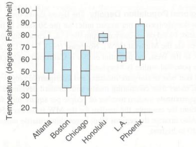
City Temperatures The boxplot shows temperatures for six cities. Each city's boxplot was made from 12 temperatures: the aver-age monthly temperature over a period of years. Which city tends to be warmest? Which city has the most variation in temperatures? Compare the temperatures of the cities by interpreting the boxplots. If temperature were the only factor to consider, which city you would choose to live in, and why?
Expert Solution & Answer
Want to see the full answer?
Check out a sample textbook solution
Students have asked these similar questions
Selon une économiste d’une société financière, les dépenses moyennes pour « meubles et appareils de maison » ont été moins importantes pour les ménages de la région de Montréal, que celles de la région de Québec.
Un échantillon aléatoire de 14 ménages pour la région de Montréal et de 16 ménages pour la région Québec est tiré et donne les données suivantes, en ce qui a trait aux dépenses pour ce secteur d’activité économique.
On suppose que les données de chaque population sont distribuées selon une loi normale.
Nous sommes intéressé à connaitre si les variances des populations sont égales.a) Faites le test d’hypothèse sur deux variances approprié au seuil de signification de 1 %. Inclure les informations suivantes :
i. Hypothèse / Identification des populationsii. Valeur(s) critique(s) de Fiii. Règle de décisioniv. Valeur du rapport Fv. Décision et conclusion
b) A partir des résultats obtenus en a), est-ce que l’hypothèse d’égalité des variances pour cette…
According to an economist from a financial company, the average expenditures on "furniture and household appliances" have been lower for households in the Montreal area than those in the Quebec region.
A random sample of 14 households from the Montreal region and 16 households from the Quebec region was taken, providing the following data regarding expenditures in this economic sector.
It is assumed that the data from each population are distributed normally.
We are interested in knowing if the variances of the populations are equal. a) Perform the appropriate hypothesis test on two variances at a significance level of 1%. Include the following information:
i. Hypothesis / Identification of populations ii. Critical F-value(s) iii. Decision rule iv. F-ratio value v. Decision and conclusion
b) Based on the results obtained in a), is the hypothesis of equal variances for this socio-economic characteristic measured in these two populations upheld?
c) Based on the results obtained in a),…
A major company in the Montreal area, offering a range of engineering services from project preparation to construction execution, and industrial project management, wants to ensure that the individuals who are responsible for project cost estimation and bid preparation demonstrate a certain uniformity in their estimates. The head of civil engineering and municipal services decided to structure an experimental plan to detect if there could be significant differences in project evaluation.
Seven projects were selected, each of which had to be evaluated by each of the two estimators, with the order of the projects submitted being random. The obtained estimates are presented in the table below.
a) Complete the table above by calculating: i. The differences (A-B) ii. The sum of the differences iii. The mean of the differences iv. The standard deviation of the differences
b) What is the value of the t-statistic?
c) What is the critical t-value for this test at a significance level of 1%?…
Chapter 3 Solutions
Introductory Statistics (2nd Edition)
Ch. 3 - Earnings A sociologist says, “Typically, men in...Ch. 3 - Houses A real estate agent claims that all things...Ch. 3 - Age of CEOs (Example) the histogram shows the ages...Ch. 3 - Televisions The histogram shows the number of...Ch. 3 - Billionaires According to Forbes.com, the numbers...Ch. 3 - Billionaires According to Forbes.com, the numbers...Ch. 3 - Paid Vacation Days (Example 2) This list...Ch. 3 - Children of First Ladies This list represents the...Ch. 3 - Ages of Presidents at Inauguration At their...Ch. 3 - Ages of Chief Justices at Installation At their...
Ch. 3 - Weight Loss (Example 3) The table shows Minitab...Ch. 3 - Education of Father and Mother The table shows...Ch. 3 - Surfing College students and surfers Rex Robinson...Ch. 3 - Eating Out College student Jacqueline Loya asked a...Ch. 3 - Real state price (Example) look at the two...Ch. 3 - Dice The histogram contain data with a range of 1...Ch. 3 - Birth Weights (Example 5) The mean birth weigh for...Ch. 3 - Birth Length The mean birth length for U.S....Ch. 3 - Children’s Ages (Example 6) Mrs. Johnson’s...Ch. 3 - Pay Rate in Different Currencies The pay rates for...Ch. 3 - Olympics In the most recent summer Olympics, do...Ch. 3 - Weights Suppose you have a data set with the...Ch. 3 - Brain Size The brain size (in hundreds of...Ch. 3 - Happiness A survey on StatCrunch asked people to...Ch. 3 - Drinkers The number of alcoholic drinks per week...Ch. 3 - Prob. 26SECh. 3 - Violent Crime: West (Example 7) In 2011, the mean...Ch. 3 - Violent Crime: East In 2011, the mean rate of...Ch. 3 - Property Crime (Example 8) In 2011, the mean...Ch. 3 - Property Crime In 2011, the mean property crime...Ch. 3 - Heights and z-Scores The dotplot shows heights of...Ch. 3 - Heights Refer to the dotplot in the previous...Ch. 3 - Unusual IQs (Example 9) Wechsler IQ tests have a...Ch. 3 - Lengths of Pregnancy Distributions of gestation...Ch. 3 - Low-Birth-Weight Babies (Example 10) Babies born...Ch. 3 - Birth Lengths Babies born after 40 weeks gestation...Ch. 3 - Women's Heights Assume that women's heights have a...Ch. 3 - SATs The quantitative portion of the SAT exam has...Ch. 3 - Name two measures of the center of a distribution,...Ch. 3 - Name two measures of the variation of a...Ch. 3 - Pixar Animated Movies (Example 11) The ten...Ch. 3 - DreamWorks Animated Movies The ten top-grossing...Ch. 3 - Pixar Animated Movies Again (Example 12) Find the...Ch. 3 - Dreamworks Animated Movies Find the median and...Ch. 3 - Prob. 45SECh. 3 - Drinks The number of alcoholic drinks per week is...Ch. 3 - Outliers a. In your own words, describe to someone...Ch. 3 - Center and Variation When you are comparing two...Ch. 3 - An Error A dieter recorded the number of calories...Ch. 3 - Baseball Strike In 1994, Major League Baseball...Ch. 3 - Heads The graphs show the circumferences of heads...Ch. 3 - House Prices The graphs show the house prices (in...Ch. 3 - Shoes (Example 14) The histograms show the number...Ch. 3 - Tax Rate A StatCrunch survey asked people what...Ch. 3 - Regional Population Density The figure shows the...Ch. 3 - Property Crime Rates The boxplot shows the...Ch. 3 - City Temperatures The boxplot shows temperatures...Ch. 3 - Brain Size The boxplots show the brain size (in...Ch. 3 - Matching Boxplots and Histograms a. Report the...Ch. 3 - Matching Boxplots and Histograms Match each of the...Ch. 3 - Sleep Time of Animals Data at this text's website...Ch. 3 - BA Percentage The data show the percentage of...Ch. 3 - Tall Buildings The dotplot shows the distribution...Ch. 3 - Passing the Bar Exam The dotplot shows the...Ch. 3 - Exam Scores The five-number summary for a...Ch. 3 - Exam Scores The five-number summary for a...Ch. 3 - Death Row: South (Example 15) The table shows the...Ch. 3 - Death Row: West The table shows the numbers of...Ch. 3 - Head Circumference (Example 16) Following are head...Ch. 3 - Heights of Sons and Dads The data at this text’s...Ch. 3 - Final Exam Grades The data that follow are final...Ch. 3 - Speeding Tickets College students Diane Glover and...Ch. 3 - Heights The following graph shows the heights for...Ch. 3 - Marathon Times The following histogram of marathon...Ch. 3 - Soda Consumption A StatCrunch survey asked people...Ch. 3 - Holiday Spending A StatCrunch survey asked people...Ch. 3 - a. State an approximate value for the mean height...Ch. 3 - Ideal Family In 2012, the General Social Survey...Ch. 3 - For exercises 3.85 through 3.88, construct two...Ch. 3 - For exercises 3.85 through 3.88, construct two...Ch. 3 - For exercises 3.85 through 3.88, construct two...Ch. 3 - 3.79-3.82 construct two sets of numbers with at...Ch. 3 - Population Density Data were recorded for each of...Ch. 3 - Population Increase Data were recorded for each of...Ch. 3 - Prob. 85CRECh. 3 - Eating Out, Again College student Jacqueline Loya...Ch. 3 - Study Hours A group of 50 statistics students, 25...Ch. 3 - Driving Accidents College student Sandy Hudson...Ch. 3 - Exam Scores An exam has a mean of 70 and a...Ch. 3 - Boys’ Heights Three-year-old boys in the United...Ch. 3 - SAT and ACT Scores Quantitative SAT scores have a...Ch. 3 - Children’s Heights Mrs. Diaz has two children: a...Ch. 3 - Students’ Ages Here are the ages of some students...Ch. 3 - House Prices The figure, which is from data taken...
Knowledge Booster


Learn more about
Need a deep-dive on the concept behind this application? Look no further. Learn more about this topic, statistics and related others by exploring similar questions and additional content below.Similar questions
- Compute the relative risk of falling for the two groups (did not stop walking vs. did stop). State/interpret your result verbally.arrow_forwardMicrosoft Excel include formulasarrow_forwardQuestion 1 The data shown in Table 1 are and R values for 24 samples of size n = 5 taken from a process producing bearings. The measurements are made on the inside diameter of the bearing, with only the last three decimals recorded (i.e., 34.5 should be 0.50345). Table 1: Bearing Diameter Data Sample Number I R Sample Number I R 1 34.5 3 13 35.4 8 2 34.2 4 14 34.0 6 3 31.6 4 15 37.1 5 4 31.5 4 16 34.9 7 5 35.0 5 17 33.5 4 6 34.1 6 18 31.7 3 7 32.6 4 19 34.0 8 8 33.8 3 20 35.1 9 34.8 7 21 33.7 2 10 33.6 8 22 32.8 1 11 31.9 3 23 33.5 3 12 38.6 9 24 34.2 2 (a) Set up and R charts on this process. Does the process seem to be in statistical control? If necessary, revise the trial control limits. [15 pts] (b) If specifications on this diameter are 0.5030±0.0010, find the percentage of nonconforming bearings pro- duced by this process. Assume that diameter is normally distributed. [10 pts] 1arrow_forward
- 4. (5 pts) Conduct a chi-square contingency test (test of independence) to assess whether there is an association between the behavior of the elderly person (did not stop to talk, did stop to talk) and their likelihood of falling. Below, please state your null and alternative hypotheses, calculate your expected values and write them in the table, compute the test statistic, test the null by comparing your test statistic to the critical value in Table A (p. 713-714) of your textbook and/or estimating the P-value, and provide your conclusions in written form. Make sure to show your work. Did not stop walking to talk Stopped walking to talk Suffered a fall 12 11 Totals 23 Did not suffer a fall | 2 Totals 35 37 14 46 60 Tarrow_forwardQuestion 2 Parts manufactured by an injection molding process are subjected to a compressive strength test. Twenty samples of five parts each are collected, and the compressive strengths (in psi) are shown in Table 2. Table 2: Strength Data for Question 2 Sample Number x1 x2 23 x4 x5 R 1 83.0 2 88.6 78.3 78.8 3 85.7 75.8 84.3 81.2 78.7 75.7 77.0 71.0 84.2 81.0 79.1 7.3 80.2 17.6 75.2 80.4 10.4 4 80.8 74.4 82.5 74.1 75.7 77.5 8.4 5 83.4 78.4 82.6 78.2 78.9 80.3 5.2 File Preview 6 75.3 79.9 87.3 89.7 81.8 82.8 14.5 7 74.5 78.0 80.8 73.4 79.7 77.3 7.4 8 79.2 84.4 81.5 86.0 74.5 81.1 11.4 9 80.5 86.2 76.2 64.1 80.2 81.4 9.9 10 75.7 75.2 71.1 82.1 74.3 75.7 10.9 11 80.0 81.5 78.4 73.8 78.1 78.4 7.7 12 80.6 81.8 79.3 73.8 81.7 79.4 8.0 13 82.7 81.3 79.1 82.0 79.5 80.9 3.6 14 79.2 74.9 78.6 77.7 75.3 77.1 4.3 15 85.5 82.1 82.8 73.4 71.7 79.1 13.8 16 78.8 79.6 80.2 79.1 80.8 79.7 2.0 17 82.1 78.2 18 84.5 76.9 75.5 83.5 81.2 19 79.0 77.8 20 84.5 73.1 78.2 82.1 79.2 81.1 7.6 81.2 84.4 81.6 80.8…arrow_forwardName: Lab Time: Quiz 7 & 8 (Take Home) - due Wednesday, Feb. 26 Contingency Analysis (Ch. 9) In lab 5, part 3, you will create a mosaic plot and conducted a chi-square contingency test to evaluate whether elderly patients who did not stop walking to talk (vs. those who did stop) were more likely to suffer a fall in the next six months. I have tabulated the data below. Answer the questions below. Please show your calculations on this or a separate sheet. Did not stop walking to talk Stopped walking to talk Totals Suffered a fall Did not suffer a fall Totals 12 11 23 2 35 37 14 14 46 60 Quiz 7: 1. (2 pts) Compute the odds of falling for each group. Compute the odds ratio for those who did not stop walking vs. those who did stop walking. Interpret your result verbally.arrow_forward
- Solve please and thank you!arrow_forward7. In a 2011 article, M. Radelet and G. Pierce reported a logistic prediction equation for the death penalty verdicts in North Carolina. Let Y denote whether a subject convicted of murder received the death penalty (1=yes), for the defendant's race h (h1, black; h = 2, white), victim's race i (i = 1, black; i = 2, white), and number of additional factors j (j = 0, 1, 2). For the model logit[P(Y = 1)] = a + ß₁₂ + By + B²², they reported = -5.26, D â BD = 0, BD = 0.17, BY = 0, BY = 0.91, B = 0, B = 2.02, B = 3.98. (a) Estimate the probability of receiving the death penalty for the group most likely to receive it. [4 pts] (b) If, instead, parameters used constraints 3D = BY = 35 = 0, report the esti- mates. [3 pts] h (c) If, instead, parameters used constraints Σ₁ = Σ₁ BY = Σ; B = 0, report the estimates. [3 pts] Hint the probabilities, odds and odds ratios do not change with constraints.arrow_forwardSolve please and thank you!arrow_forward
- Solve please and thank you!arrow_forwardQuestion 1:We want to evaluate the impact on the monetary economy for a company of two types of strategy (competitive strategy, cooperative strategy) adopted by buyers.Competitive strategy: strategy characterized by firm behavior aimed at obtaining concessions from the buyer.Cooperative strategy: a strategy based on a problem-solving negotiating attitude, with a high level of trust and cooperation.A random sample of 17 buyers took part in a negotiation experiment in which 9 buyers adopted the competitive strategy, and the other 8 the cooperative strategy. The savings obtained for each group of buyers are presented in the pdf that i sent: For this problem, we assume that the samples are random and come from two normal populations of unknown but equal variances.According to the theory, the average saving of buyers adopting a competitive strategy will be lower than that of buyers adopting a cooperative strategy.a) Specify the population identifications and the hypotheses H0 and H1…arrow_forwardYou assume that the annual incomes for certain workers are normal with a mean of $28,500 and a standard deviation of $2,400. What’s the chance that a randomly selected employee makes more than $30,000?What’s the chance that 36 randomly selected employees make more than $30,000, on average?arrow_forward
arrow_back_ios
SEE MORE QUESTIONS
arrow_forward_ios
Recommended textbooks for you
 Holt Mcdougal Larson Pre-algebra: Student Edition...AlgebraISBN:9780547587776Author:HOLT MCDOUGALPublisher:HOLT MCDOUGAL
 Glencoe Algebra 1, Student Edition, 9780079039897...AlgebraISBN:9780079039897Author:CarterPublisher:McGraw Hill
 Algebra: Structure And Method, Book 1AlgebraISBN:9780395977224Author:Richard G. Brown, Mary P. Dolciani, Robert H. Sorgenfrey, William L. ColePublisher:McDougal Littell
 Big Ideas Math A Bridge To Success Algebra 1: Stu...AlgebraISBN:9781680331141Author:HOUGHTON MIFFLIN HARCOURTPublisher:Houghton Mifflin Harcourt
 College Algebra (MindTap Course List)AlgebraISBN:9781305652231Author:R. David Gustafson, Jeff HughesPublisher:Cengage Learning
Holt Mcdougal Larson Pre-algebra: Student Edition...
Algebra
ISBN:9780547587776
Author:HOLT MCDOUGAL
Publisher:HOLT MCDOUGAL
Glencoe Algebra 1, Student Edition, 9780079039897...
Algebra
ISBN:9780079039897
Author:Carter
Publisher:McGraw Hill
Algebra: Structure And Method, Book 1
Algebra
ISBN:9780395977224
Author:Richard G. Brown, Mary P. Dolciani, Robert H. Sorgenfrey, William L. Cole
Publisher:McDougal Littell
Big Ideas Math A Bridge To Success Algebra 1: Stu...
Algebra
ISBN:9781680331141
Author:HOUGHTON MIFFLIN HARCOURT
Publisher:Houghton Mifflin Harcourt
College Algebra (MindTap Course List)
Algebra
ISBN:9781305652231
Author:R. David Gustafson, Jeff Hughes
Publisher:Cengage Learning
Statistics 4.1 Point Estimators; Author: Dr. Jack L. Jackson II;https://www.youtube.com/watch?v=2MrI0J8XCEE;License: Standard YouTube License, CC-BY
Statistics 101: Point Estimators; Author: Brandon Foltz;https://www.youtube.com/watch?v=4v41z3HwLaM;License: Standard YouTube License, CC-BY
Central limit theorem; Author: 365 Data Science;https://www.youtube.com/watch?v=b5xQmk9veZ4;License: Standard YouTube License, CC-BY
Point Estimate Definition & Example; Author: Prof. Essa;https://www.youtube.com/watch?v=OTVwtvQmSn0;License: Standard Youtube License
Point Estimation; Author: Vamsidhar Ambatipudi;https://www.youtube.com/watch?v=flqhlM2bZWc;License: Standard Youtube License