
Videos
The dynamics of a forced spring-mass-damper system can be represented by the following second-order ODE:
where
(a)
To calculate: The displacement and velocity as a function of time for linear system where
Answer to Problem 49P
Solution:
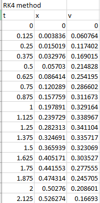
The first few solutions for displacement and velocity as a function of time for liner system is,
| t | x | v |
| 0 | 0 | 0 |
| 0.125 | 0.003836 | 0.060764 |
| 0.25 | 0.015019 | 0.117402 |
| 0.375 | 0.032976 | 0.169015 |
| 0.5 | 0.05703 | 0.214828 |
| 0.625 | 0.086414 | 0.254195 |
| 0.75 | 0.120289 | 0.286602 |
| 0.875 | 0.157759 | 0.311673 |
| 1 | 0.197891 | 0.329164 |
| 1.125 | 0.239729 | 0.338967 |
| 1.25 | 0.282313 | 0.341104 |
| 1.375 | 0.324691 | 0.335717 |
| 1.5 | 0.365939 | 0.323069 |
| 1.625 | 0.405171 | 0.303527 |
| 1.75 | 0.441553 | 0.277555 |
| 1.875 | 0.474314 | 0.245705 |
| 2 | 0.50276 | 0.208601 |
| 2.125 | 0.526274 | 0.16693 |
| 2.25 | 0.544332 | 0.121428 |
| 2.375 | 0.556503 | 0.072863 |
| 2.5 | 0.562454 | 0.02203 |
| 2.625 | 0.56195 | -0.03027 |
| 2.75 | 0.554859 | -0.08324 |
| 2.875 | 0.541146 | -0.13608 |
| 3 | 0.520874 | -0.18805 |
| 3.125 | 0.494199 | -0.23842 |
| 3.25 | 0.461364 | -0.28651 |
| 3.375 | 0.422694 | -0.33168 |
| 3.5 | 0.378588 | -0.37339 |
| 3.625 | 0.329513 | -0.41112 |
| 3.75 | 0.275993 | -0.44444 |
| 3.875 | 0.218601 | -0.47301 |
| 4 | 0.157952 | -0.49653 |
| 4.125 | 0.094688 | -0.5148 |
| 4.25 | 0.029475 | -0.52771 |
| 4.375 | -0.03701 | -0.53518 |
| 4.5 | -0.1041 | -0.53725 |
| 4.625 | -0.1711 | -0.53399 |
| 4.75 | -0.23738 | -0.52558 |
| 4.875 | -0.30229 | -0.51221 |
| 5 | -0.36524 | -0.49416 |
Explanation of Solution
Given Information:
The dynamic of a forced spring-mass-damper system is given as,
The values,
The initial condition,
Formula used:
The fourth-order RK method for
Where,
Calculation:
Consider the dynamic of a forced spring-mass-damper system,
As
Divide both the sides of above equation by m,
Now, substitute the values
For linear, substitute
Use VBA code for RK4 method as below to solve for x and v,
Code:
Output:
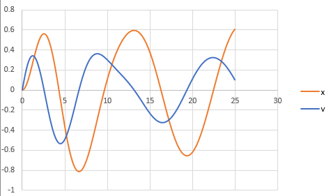
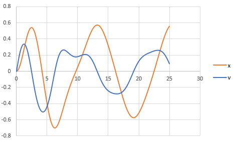
To draw the graph of the above results, follow the steps in excel sheet as given below,
Step 1: Select the cell from A4 to A205 and cell B4 to B205. Then, go to the Insert and select the scatter with smooth lines from the chart.
Step 2: Select the cell from A4 to A205 and cell C4 to C205. Then, go to the Insert and select the scatter with smooth lines from the chart.
Step 3: Select one of the graphs and paste it on another graph to merge the graphs.
The graph obtained is,
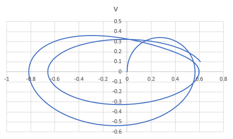
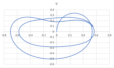
And, to draw the phase plane plot follow the steps as below,
Step 4: Select the column B and column C. Then, go to the Insert and select the scatter with smooth lines from the chart.
The graph obtained is,
(b)
To calculate: The displacement and velocity as a function of time for non-linear system where
Answer to Problem 49P
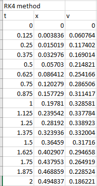
Solution:
| t | x | v |
| 0 | 0 | 0 |
| 0.125 | 0.003836 | 0.060764 |
| 0.25 | 0.015019 | 0.117402 |
| 0.375 | 0.032976 | 0.169014 |
| 0.5 | 0.05703 | 0.214821 |
| 0.625 | 0.086412 | 0.254166 |
| 0.75 | 0.120279 | 0.286506 |
| 0.875 | 0.157729 | 0.311417 |
| 1 | 0.19781 | 0.328581 |
| 1.125 | 0.239542 | 0.337784 |
| 1.25 | 0.28192 | 0.338923 |
| 1.375 | 0.323936 | 0.332004 |
| 1.5 | 0.36459 | 0.31716 |
| 1.625 | 0.402907 | 0.294658 |
| 1.75 | 0.437953 | 0.264919 |
| 1.875 | 0.468859 | 0.228524 |
| 2 | 0.494837 | 0.186221 |
| 2.125 | 0.515205 | 0.138911 |
| 2.25 | 0.5294 | 0.087637 |
| 2.375 | 0.536996 | 0.033543 |
| 2.5 | 0.537718 | -0.02217 |
| 2.625 | 0.531437 | -0.07829 |
| 2.75 | 0.518177 | -0.13366 |
| 2.875 | 0.498099 | -0.18721 |
| 3 | 0.47149 | -0.23801 |
| 3.125 | 0.438743 | -0.28531 |
| 3.25 | 0.400333 | -0.32852 |
| 3.375 | 0.3568 | -0.36723 |
| 3.5 | 0.308725 | -0.40117 |
| 3.625 | 0.256712 | -0.43023 |
| 3.75 | 0.201374 | -0.45436 |
| 3.875 | 0.143325 | -0.47361 |
| 4 | 0.083172 | -0.48804 |
| 4.125 | 0.021513 | -0.49771 |
| 4.25 | -0.04106 | -0.50268 |
| 4.375 | -0.10396 | -0.50296 |
| 4.5 | -0.1666 | -0.49854 |
| 4.625 | -0.2284 | -0.48938 |
| 4.75 | -0.28875 | -0.47544 |
| 4.875 | -0.34705 | -0.45667 |
| 5 | -0.40271 | -0.43306 |
Explanation of Solution
Given Information:
The dynamic of a forced spring-mass-damper system is given as,
The values,
And,
The initial condition,
Formula used:
The fourth-order RK method for
Where,
Calculation:
Consider the dynamic of a forced spring-mass-damper system,
As
Divide both the sides of above equation by m,
Now, substitute the values
For linear, substitute
Use VBA code for RK4 method as below to solve for x and v,
Code:
Output:
Few data are shown below,
To draw the graph of the above results, follow the steps in excel sheet as given below,
Step 1: Select the cell from A4 to A205 and cell B4 to B205. Then, go to the Insert and select the scatter with smooth lines from the chart.
Step 2: Select the cell from A4 to A205 and cell C4 to C205. Then, go to the Insert and select the scatter with smooth lines from the chart.
Step 3: Select one of the graphs and paste it on another graph to merge the graphs.
The graph obtained is,
And, to draw the phase plane plot follow the steps as below,
Step 4: Select the column B and column C. Then, go to the Insert and select the scatter with smooth lines from the chart.
The graph obtained is,
Want to see more full solutions like this?
Chapter 28 Solutions
Numerical Methods for Engineers


- A straight-line H is tangent to the function g(x)=-6x-3+ 8 and passes through the point (- 4,7). Determine, the gradient of the straight-line Choose.... y-intercept of the straight-line Choose... + which of the following is the answers -1.125 -6.72 1.125 7.28 0.07 - 7.28 6.72arrow_forwardYou are required to match the correct response to each statement provided. Another term/word that can be used synonymously to Choose... gradient. A term/phrase that is associated with Arithmetic Progression. Common difference → An identity matrix can be referred to as a Choose... ÷ What is the inequality sign that represents "at most"? VIarrow_forwardAffect of sports on students linked with physical problemsarrow_forward
- 26.1. Locate and determine the order of zeros of the following functions: (a). e2z – e*, (b). z2sinhz, (c). z*cos2z, (d). z3 cosz2.arrow_forwardQ/ show that: The function feal = Se²²²+d+ is analyticarrow_forwardComplex Analysis 2 First exam Q1: Evaluate f the Figure. 23+3 z(z-i)² 2024-2025 dz, where C is the figure-eight contour shown in C₂arrow_forward
- Q/ Find the Laurent series of (2-3) cos around z = 1 2-1arrow_forward31.5. Let be the circle |+1| = 2 traversed twice in the clockwise direction. Evaluate dz (22 + 2)²arrow_forwardUsing FDF, BDF, and CDF, find the first derivative; 1. The distance x of a runner from a fixed point is measured (in meters) at an interval of half a second. The data obtained is: t 0 x 0 0.5 3.65 1.0 1.5 2.0 6.80 9.90 12.15 Use CDF to approximate the runner's velocity at times t = 0.5s and t = 1.5s 2. Using FDF, BDF, and CDF, find the first derivative of f(x)=x Inx for an input of 2 assuming a step size of 1. Calculate using Analytical Solution and Absolute Relative Error: = True Value - Approximate Value| x100 True Value 3. Given the data below where f(x) sin (3x), estimate f(1.5) using Langrage Interpolation. x 1 1.3 1.6 1.9 2.2 f(x) 0.14 -0.69 -0.99 -0.55 0.31 4. The vertical distance covered by a rocket from t=8 to t=30 seconds is given by: 30 x = Loo (2000ln 140000 140000 - 2100 9.8t) dt Using the Trapezoidal Rule, n=2, find the distance covered. 5. Use Simpson's 1/3 and 3/8 Rule to approximate for sin x dx. Compare the results for n=4 and n=8arrow_forward
- 1. A Blue Whale's resting heart rate has period that happens to be approximately equal to 2π. A typical ECG of a whale's heartbeat over one period may be approximated by the function, f(x) = 0.005x4 2 0.005x³-0.364x² + 1.27x on the interval [0, 27]. Find an nth-order Fourier approximation to the Blue Whale's heartbeat, where n ≥ 3 is different from that used in any other posts on this topic, to generate a periodic function that can be used to model its heartbeat, and graph your result. Be sure to include your chosen value of n in your Subject Heading.arrow_forward7. The demand for a product, in dollars, is p = D(x) = 1000 -0.5 -0.0002x² 1 Find the consumer surplus when the sales level is 200. [Hints: Let pm be the market price when xm units of product are sold. Then the consumer surplus can be calculated by foam (D(x) — pm) dx]arrow_forward4. Find the general solution and the definite solution for the following differential equations: (a) +10y=15, y(0) = 0; (b) 2 + 4y = 6, y(0) =arrow_forward
 Advanced Engineering MathematicsAdvanced MathISBN:9780470458365Author:Erwin KreyszigPublisher:Wiley, John & Sons, Incorporated
 Numerical Methods for EngineersAdvanced MathISBN:9780073397924Author:Steven C. Chapra Dr., Raymond P. CanalePublisher:McGraw-Hill Education
 Introductory Mathematics for Engineering Applicat...Advanced MathISBN:9781118141809Author:Nathan KlingbeilPublisher:WILEY
 Mathematics For Machine TechnologyAdvanced MathISBN:9781337798310Author:Peterson, John.Publisher:Cengage Learning,
