
Concept explainers
Videos
The basic
Where
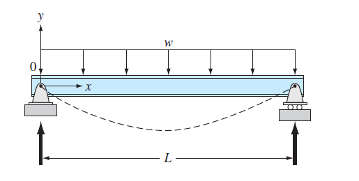
FIGURE P28.27
(a)
To calculate: The deflection of the beam by the finite-difference method with
Answer to Problem 27P
Solution:
The deflection of the beam by the finite-difference method is,
| x | y | y-Analytical |
| 0 | 0 | 0 |
| 24 | ||
| 48 | ||
| 72 | ||
| 96 | ||
| 120 | 0 | 0 |
Explanation of Solution
Given Information:
The differential equation for the elastic curve for a uniformly loaded beam is given as,
Formula to find analytical value,
Where,
The modulus of elasticity,
The moment of inertia,
The values,
Formula used:
The conversion formula,
The value of second order derivative by finite difference method is given as,
Calculation:
Consider the equation,
Rewrite the above equation as,
Substitute the values,
Now, the second order derivative by finite difference method gives,
Therefore,
Put
The boundary condition is,
Put
Substitute
Put
Substitute
Put
Substitute
The matrix form of the above equations is given as below,
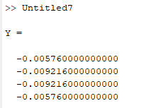
Use MATLAB to find the solution of the above system as below,
Code:
%Write the matrix
A=[-2 1 0 0; 1 -2 1 0; 0 1 -2 1; 0 0 1 -2];
%write the values of rhs
b=[0.002304 0.003456 0.003456 0.002304]';
%find the result
Y=A\b
Output:
Now, for the analytical value, consider the equation
Substitute the values,
Use excel to find the values of y at different values of x as below,
Step 1: Name the column A as x and go to column A2 and put 0 then go to column A3 and write the formula as,
=A2+24
Then, Press enter and drag the column up to
Step 2: Now name the column B as y and go to column B2 andwrite the formula as,
=2.89236*10^(-10)*A2*(120*A2^2-0.5*A2^3-864000)
Step 3: Press enter and drag the column up to
The result obtained as,
| x | y-Analytical |
| 0 | 0 |
| 24 | |
| 48 | |
| 72 | |
| 96 | |
| 120 | 0 |
(b)
To calculate: The deflection of the beam by the shooting method with
Answer to Problem 27P
Solution:
A few values of deflection of the beam by the shooting method is,
| x | y | z |
| 0 | 0 | -1.6E-06 |
| 0.25 | -4.1E-07 | -1.6E-06 |
| 0.5 | -8.2E-07 | -1.6E-06 |
| 0.75 | -1.2E-06 | -1.6E-06 |
| 1 | -1.6E-06 | -1.6E-06 |
| 1.25 | -2E-06 | -1.5E-06 |
| 1.5 | -2.4E-06 | -1.4E-06 |
| 1.75 | -2.8E-06 | -1.4E-06 |
| 2 | -3.2E-06 | -1.3E-06 |
| 2.25 | -3.5E-06 | -1.2E-06 |
| 2.5 | -3.8E-06 | -1.1E-06 |
| 2.75 | -4.1E-06 | -1E-06 |
| 3 | -4.4E-06 | -9E-07 |
Explanation of Solution
Given Information:
The differential equation for the elastic curve for a uniformly loaded beam is given as,
Formula to find analytical value,
Where,
The modulus of elasticity,
The moment of inertia,
The values,
Formula used:
The conversion formula,
Calculation:
Consider the equation,
Rewrite the equation as,
Assume
Substitute the values,
Use VBA program as below to solve the above differential equation as below,
Code:
OptionExplicit
'Create a function find
Subfind()
'declare the variables as integer
Dim n AsInteger, j AsInteger
'declare the variables as double
DimdydxAsDouble, x AsDouble, dy2dx AsDouble, yanalAsDouble, E AsDouble, I AsDouble, w AsDouble, L AsDouble
DimolddydxAsDouble, oldy AsDouble, y AsDouble, h AsDouble
'Set the values of the variables
E =30000
I =800
w =1
L =10
y =0
x =0
h =0.25
dydx=0
'store dydx and analytical solution
dydx= caldydx(w, E, I, L, x)
yanal= caly(w, E, I, L, x)
'use for loop to determine different value of y and y analytical
For j =1 To41
'store the value of y at oldy and dydx in olddydx
oldy = y
olddydx= dydx
'Store d2ydx, dydx and analytical solution
dy2dx = caldy2dx(w, E, I, L, x)
dydx= caldydx(w, E, I, L, x)
yanal= caly(w, E, I, L, x)
'move to the cell b3
Range("b1"). Select
ActiveCell.Value="shooting method"
'Assign name to the columns
ActiveCell.Offset(1,0). Select
ActiveCell.Value="x"
ActiveCell.Offset(0,1). Select
ActiveCell.Value="y"
ActiveCell.Offset(0,1). Select
ActiveCell.Value="z"
ActiveCell.Offset(0,1). Select
ActiveCell.Value="dy2dx"
ActiveCell.Offset(0,1). Select
ActiveCell.Value="y-anal"
'dislay values in cell
Range("b2"). Select
ActiveCell.Offset(j,0). Select
ActiveCell.Value= x
ActiveCell.Offset(0,1). Select
ActiveCell.Value= oldy
ActiveCell.Offset(0,1). Select
ActiveCell.Value= dydx
ActiveCell.Offset(0,1). Select
ActiveCell.Value= dy2dx
ActiveCell.Offset(0,1). Select
ActiveCell.Value= yanal
'Write the next value of x
x = x + h
'Write the next value of y by euler method
y = oldy + olddydx* h
Next
EndSub
'Define d2ydx function
Function caldy2dx(w, E, I, L, x)
'Declare the variables
Dim t AsDouble
'Write the formula
t =((w * L * x)/(2* E * I))-((w * x * x)/(2* E * I))
'Store the value
caldy2dx = t
EndFunction
'Define dydx
Functioncaldydx(w, E, I, L, x)
'Declare the variables
Dim t AsDouble, c AsDouble
'Set the values
c =-0.000001648
'Write the formula
t =((w * L * x * x)/(4* E * I))-((w * x * x * x)/(6* E * I))+ c
'Store the value
caldydx= t
EndFunction
'Define the function caly for analytical value
Functioncaly(w, E, I, L, x)
'Declare the variables
Dim t AsDouble
'Write the formula
t =((w * L * x * x * x)/(12* E * I))-((w * x * x * x * x)/(24* E * I))-((w * L * L * L * x)/(24* E * I))
'Store the value
caly= t
EndFunction
Output:
| shooting method | ||||
| x | y | z | dy2dx | y-anal |
| 0 | 0 | -1.6E-06 | 0 | 0 |
| 0.25 | -4.1E-07 | -1.6E-06 | 5.08E-08 | -4.3E-07 |
| 0.5 | -8.2E-07 | -1.6E-06 | 9.9E-08 | -8.6E-07 |
| 0.75 | -1.2E-06 | -1.6E-06 | 1.45E-07 | -1.3E-06 |
| 1 | -1.6E-06 | -1.6E-06 | 1.88E-07 | -1.7E-06 |
| 1.25 | -2E-06 | -1.5E-06 | 2.28E-07 | -2.1E-06 |
| 1.5 | -2.4E-06 | -1.4E-06 | 2.66E-07 | -2.5E-06 |
| 1.75 | -2.8E-06 | -1.4E-06 | 3.01E-07 | -2.9E-06 |
| 2 | -3.2E-06 | -1.3E-06 | 3.33E-07 | -3.2E-06 |
| 2.25 | -3.5E-06 | -1.2E-06 | 3.63E-07 | -3.6E-06 |
| 2.5 | -3.8E-06 | -1.1E-06 | 3.91E-07 | -3.9E-06 |
| 2.75 | -4.1E-06 | -1E-06 | 4.15E-07 | -4.2E-06 |
| 3 | -4.4E-06 | -9E-07 | 4.38E-07 | -4.4E-06 |
| 3.25 | -4.7E-06 | -7.9E-07 | 4.57E-07 | -4.6E-06 |
| 3.5 | -4.9E-06 | -6.7E-07 | 4.74E-07 | -4.8E-06 |
| 3.75 | -5.1E-06 | -5.5E-07 | 4.88E-07 | -5E-06 |
| 4 | -5.2E-06 | -4.3E-07 | 5E-07 | -5.2E-06 |
| 4.25 | -5.4E-06 | -3E-07 | 5.09E-07 | -5.3E-06 |
| 4.5 | -5.5E-06 | -1.7E-07 | 5.16E-07 | -5.4E-06 |
| 4.75 | -5.6E-06 | -4.2E-08 | 5.2E-07 | -5.4E-06 |
| 5 | -5.6E-06 | 8.81E-08 | 5.21E-07 | -5.4E-06 |
| 5.25 | -5.6E-06 | 2.18E-07 | 5.2E-07 | -5.4E-06 |
| 5.5 | -5.6E-06 | 3.48E-07 | 5.16E-07 | -5.4E-06 |
| 5.75 | -5.5E-06 | 4.76E-07 | 5.09E-07 | -5.3E-06 |
| 6 | -5.4E-06 | 6.02E-07 | 5E-07 | -5.2E-06 |
| 6.25 | -5.3E-06 | 7.26E-07 | 4.88E-07 | -5E-06 |
| 6.5 | -5.2E-06 | 8.46E-07 | 4.74E-07 | -4.8E-06 |
| 6.75 | -5E-06 | 9.62E-07 | 4.57E-07 | -4.6E-06 |
| 7 | -4.8E-06 | 1.07E-06 | 4.38E-07 | -4.4E-06 |
| 7.25 | -4.5E-06 | 1.18E-06 | 4.15E-07 | -4.2E-06 |
| 7.5 | -4.3E-06 | 1.28E-06 | 3.91E-07 | -3.9E-06 |
| 7.75 | -4E-06 | 1.38E-06 | 3.63E-07 | -3.6E-06 |
| 8 | -3.7E-06 | 1.46E-06 | 3.33E-07 | -3.2E-06 |
| 8.25 | -3.3E-06 | 1.54E-06 | 3.01E-07 | -2.9E-06 |
| 8.5 | -3E-06 | 1.61E-06 | 2.66E-07 | -2.5E-06 |
| 8.75 | -2.6E-06 | 1.68E-06 | 2.28E-07 | -2.1E-06 |
| 9 | -2.2E-06 | 1.73E-06 | 1.88E-07 | -1.7E-06 |
| 9.25 | -1.7E-06 | 1.77E-06 | 1.45E-07 | -1.3E-06 |
| 9.5 | -1.3E-06 | 1.8E-06 | 9.9E-08 | -8.6E-07 |
| 9.75 | -8.7E-07 | 1.82E-06 | 5.08E-08 | -4.3E-07 |
| 10 | -4.2E-07 | 1.82E-06 | 0 | 0 |
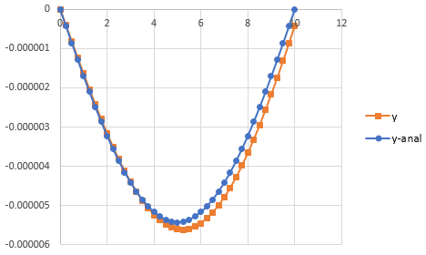
Now, to draw the graph of y and y-analytical follow the step as below,
Step 1: Select the cell from B2 to B43 and cell C2 to C43. Then, go to the Insert and select the scatter with smooth lines from the chart.
Step 2: Select the cell from B2 to B43 and cell F2 to F43. Then, go to the Insert and select the scatter with smooth lines from the chart.
Step 3: Select one of the graphs and paste it on another graph to merge the graphs.
The graph obtained is,
Want to see more full solutions like this?
Chapter 28 Solutions
Numerical Methods for Engineers
Additional Math Textbook Solutions
Probability And Statistical Inference (10th Edition)
Introductory Statistics
Finite Mathematics for Business, Economics, Life Sciences and Social Sciences
Elementary and Intermediate Algebra: Concepts and Applications (7th Edition)
A First Course in Probability (10th Edition)
Precalculus: A Unit Circle Approach (3rd Edition)


- 3. A spreadsheet consists of cells indexed by a row and a column. Each cell contains either a value or a formula that depends on the values of other cells. (a) Describe a graph, digraph, or network that models an arbitrary spreadsheet and allows you to answer the remaining parts of this question. (b) Explain, by referring to the graph, digraph, or network, when it is possible to change the value of cell x without changing the value of cell y. (c) Explain, by referring to the graph, digraph, or network, when it is possible to calculate the values of all cells in the spreadsheet. Consider the following spreadsheet with 5 rows, 7 columns, and 35 cells. For exam- ple, cell el contains a value, whereas cell al contains a formula that depends on the values cells el and 95. a b с d e f g 1 el+g5 al-c5 110 al+cl 180 f5-el c1+c2 2 al+bl a2+c4 240 a2+c2 120 f5-e2 e3+e5 3 a2+b2 a3-c3 100 a3+c1 200 f5-e3 f1+f2 4 a3+b3 a4+c2 220 a4+c2 100 f5-e4 f3+f4 5 a4+b4 a5-c1 130 a5+c5 120 g3+g4 gl+g2 (d) Can…arrow_forwardSolution: Solution: 7.2 2x²+5x-3. Diagram: till sh one The Steps the same technique as in 4 and 5) above to factor the following Show all the Steps. "Diagram, (2) 03) But (be Wha x+2 3arrow_forwardQ/ solving Laplace equation on Rectangular Rejon a xx+uyy = o u (x, 0) = u(x,2) = 0 u (o,y) = y (1,y) = 27arrow_forward
- Q / solving ha place equation a x x + u y y = 0 u (x, 0)=0 u ( x, 2) = 10 u (o,y) = 4 (119)=0 и on Rectangular Rejonarrow_forwardConjecture Let x and y be integers. If x is even and y is odd, then xy is even. Try some examples. Does the conjecture seem to be true or false?arrow_forwardSOLVE ONLY FOR (L) (M) AND (O)arrow_forward
- File Preview A gardener has ten different potted plants, and they are spraying the plants with doses of Tertizers. Plants can receive zero or more doses in a session. In the following, we count each possible number of doses the ten plants can receive (the order of spraying in a session does not matter). (a) How many ways are there if there were twelve total doses of a single type of fertilizer? (b) How many ways are there if there are six total doses of a single type of fertilizer, each plant receives no more than one dose? (c) How many ways are there if is was one dose of each of six types of fertilizers? (d) How many ways are there if there are four doses of fertilizer #1 and eight doses of fertilizer #2? (e) How many ways are there if there are four doses of fertilizer #1 and eight doses of fertilizer #2, and each plant receives no more than one dose of fertilizer #1? (f) How many ways are there to do two sessions of spraying, where each plant receives at most two doses total?arrow_forwarda) x(t) = rect(t − 3) b) x(t) = −3t rect(t) . c) x(t) = 2te 3u1(t) d) x(t) = e−2|t| 2. Sketch the magnitude and phase spectrum for the four signals in Problem (1).arrow_forwardG(x) = dt 1+√t (x > 0). Find G' (9)arrow_forward
- What is the area of this figure? 7 mi 3 mi 8 mi 5 mi 2 mi 6 mi 3 mi 9 miarrow_forwardQ/ Solving Laplace equation on a Rectangular Rejon uxxuyy = o u(x, 0) = f(x) исх, 6) = д(х) b) u Co,y) = u(a,y) = =0arrow_forwardQ/solve the heat equation initial-boundary-value problem- u+= 2uxx 4 (x10) = x+\ u (o,t) = ux (4,t) = 0arrow_forward
 College Algebra (MindTap Course List)AlgebraISBN:9781305652231Author:R. David Gustafson, Jeff HughesPublisher:Cengage Learning