Elementary Statistics 2nd Edition
2nd Edition
ISBN: 9781259724275
Author: William Navidi, Barry Monk
Publisher: McGraw-Hill Education
expand_more
expand_more
format_list_bulleted
Concept explainers
Videos
Textbook Question
Chapter 2.4, Problem 12E
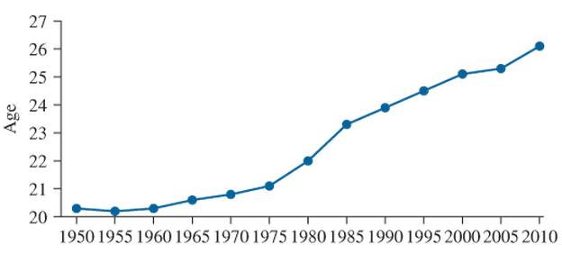
Age at marriage: Data compiled by the U.S. Census Bureau suggests that the age at which women first marry has increased over time. The following time-series plot presents the average age at which women first marry for the years 1950—2010. Does the plot present an accurate picture of the increase, or is it misleading? Explain.
Expert Solution & Answer
Want to see the full answer?
Check out a sample textbook solution
Students have asked these similar questions
NC Current Students - North Ce X | NC Canvas Login Links - North ( X
Final Exam Comprehensive x Cengage Learning
x
WASTAT - Final Exam - STAT
→
C
webassign.net/web/Student/Assignment-Responses/submit?dep=36055360&tags=autosave#question3659890_9
Part (b)
Draw a scatter plot of the ordered pairs.
N
Life
Expectancy
Life
Expectancy
80
70
600
50
40
30
20
10
Year of
1950
1970 1990
2010 Birth
O
Life
Expectancy
Part (c)
800
70
60
50
40
30
20
10
1950
1970 1990
W
ALT
林
$
#
4
R
J7
Year of
2010 Birth
F6
4+
80
70
60
50
40
30
20
10
Year of
1950 1970 1990
2010 Birth
Life
Expectancy
Ox
800
70
60
50
40
30
20
10
Year of
1950 1970 1990 2010 Birth
hp
P.B.
KA
&
7
80
% 5
H
A
B
F10
711
N
M
K
744
PRT SC
ALT
CTRL
Harvard University
California Institute of Technology
Massachusetts Institute of Technology
Stanford University
Princeton University
University of Cambridge
University of Oxford
University of California, Berkeley
Imperial College London
Yale University
University of California, Los Angeles
University of Chicago
Johns Hopkins University
Cornell University
ETH Zurich
University of Michigan
University of Toronto
Columbia University
University of Pennsylvania
Carnegie Mellon University
University of Hong Kong
University College London
University of Washington
Duke University
Northwestern University
University of Tokyo
Georgia Institute of Technology
Pohang University of Science and Technology
University of California, Santa Barbara
University of British Columbia
University of North Carolina at Chapel Hill
University of California, San Diego
University of Illinois at Urbana-Champaign
National University of Singapore
McGill…
Name
Harvard University
California Institute of Technology
Massachusetts Institute of Technology
Stanford University
Princeton University
University of Cambridge
University of Oxford
University of California, Berkeley
Imperial College London
Yale University
University of California, Los Angeles
University of Chicago
Johns Hopkins University
Cornell University
ETH Zurich
University of Michigan
University of Toronto
Columbia University
University of Pennsylvania
Carnegie Mellon University
University of Hong Kong
University College London
University of Washington
Duke University
Northwestern University
University of Tokyo
Georgia Institute of Technology
Pohang University of Science and Technology
University of California, Santa Barbara
University of British Columbia
University of North Carolina at Chapel Hill
University of California, San Diego
University of Illinois at Urbana-Champaign
National University of Singapore…
Chapter 2 Solutions
Elementary Statistics 2nd Edition
Ch. 2.1 - In Exercises 5-8, fill in each blank with the...Ch. 2.1 - In Exercises 5-8, fill in each blank with the...Ch. 2.1 - In Exercises 5-8, fill in each blank with the...Ch. 2.1 - In Exercises 5-8, fill in each blank with the...Ch. 2.1 - In Exercises 9—12, determine whether the...Ch. 2.1 - In Exercises 9—12, determine whether the...Ch. 2.1 - In Exercises 9—12, determine whether the...Ch. 2.1 - In Exercises 9—12, determine whether the...Ch. 2.1 - The following bar graph presents the average...Ch. 2.1 - The most common blood typing system divides human...
Ch. 2.1 - Following is a pie chart that presents the...Ch. 2.1 - Prob. 16ECh. 2.1 - Food sources: The following side-by-side bar graph...Ch. 2.1 - Prob. 18ECh. 2.1 - Prob. 19ECh. 2.1 - Popular video games: The following frequency...Ch. 2.1 - More iPods: Using the data in exercise 19:...Ch. 2.1 - Prob. 22ECh. 2.1 - Prob. 23ECh. 2.1 - World population: Following are the populations of...Ch. 2.1 - Ages of video garners: The Nielsen Company...Ch. 2.1 - How secure is your job? In a survey, employed...Ch. 2.1 - Back up your data: In a survey commissioned by the...Ch. 2.1 - Education levels: The following frequency...Ch. 2.1 - Music sales: The following frequency distribution...Ch. 2.1 - Bought a new car lately? The following table...Ch. 2.1 - Instagram followers: The following frequency...Ch. 2.1 - Smartphones: The following table present the...Ch. 2.1 - Smartphone sale: The following table presents the...Ch. 2.1 - Happy Halloween: The following table presents...Ch. 2.1 - Native languages: The following frequency...Ch. 2.2 - Prob. 5ECh. 2.2 - In Exercises 5—8, fill in each blank with the...Ch. 2.2 - In Exercises 5—8, fill in each blank with the...Ch. 2.2 - In Exercises 5—8, fill in each blank with the...Ch. 2.2 - In Exercises 9—12, determine whether the...Ch. 2.2 - In Exercises 9—12, determine whether the...Ch. 2.2 - In Exercises 9—12, determine whether the...Ch. 2.2 - In Exercises 9—12, determine whether the...Ch. 2.2 - In Exercises 13—16, classify the histogram as...Ch. 2.2 - In Exercises 13—16, classify the histogram as...Ch. 2.2 - In Exercises 13—16, classify the histogram as...Ch. 2.2 - In Exercises 13—16, classify the histogram as...Ch. 2.2 - In Exercises 17 and 18, classify the histogram as...Ch. 2.2 - In Exercises 17 and 18, classify the histogram as...Ch. 2.2 - Student heights: The following frequency histogram...Ch. 2.2 - Trained rats: Forty rats were trained to run a...Ch. 2.2 - Prob. 21ECh. 2.2 - Prob. 22ECh. 2.2 - Prob. 23ECh. 2.2 - Prob. 24ECh. 2.2 - Batting average: The following frequency...Ch. 2.2 - Batting average: The following frequency...Ch. 2.2 - Time spent playing video games: A sample of 200...Ch. 2.2 - Murder, she wrote: The following frequency...Ch. 2.2 - BMW prices: The following table presents the...Ch. 2.2 - Geysers: The geyser Old Faithful in Yellowstone...Ch. 2.2 - Hail to the chief: There have been 58 presidential...Ch. 2.2 - Internet radio: The following table presents the...Ch. 2.2 - Brothers and sisters: Thirty students in a...Ch. 2.2 - Cough, cough: The following table presents the...Ch. 2.2 - Prob. 35ECh. 2.2 - Frequency polygon: Using the data in Exercise 26:...Ch. 2.2 - Frequency polygon: Using data in Exercise 27:...Ch. 2.2 - Prob. 38ECh. 2.2 - Ogive: Using the data in Exercise 25 Compute the...Ch. 2.2 - Ogive: Using the data in Exercise 26: Compute the...Ch. 2.2 - Ogive: Using the data in Exercise 27: Compute the...Ch. 2.2 - Prob. 42ECh. 2.2 - Prob. 43ECh. 2.2 - Prob. 44ECh. 2.2 - Prob. 45ECh. 2.2 - Prob. 46ECh. 2.2 - Prob. 47ECh. 2.2 - Prob. 48ECh. 2.3 - In Exercises 3—6, fill in each blank with the...Ch. 2.3 - In Exercises 3—6, fill in each blank with the...Ch. 2.3 - In Exercises 3—6, fill in each blank with the...Ch. 2.3 - In Exercises 3—6, fill in each blank with the...Ch. 2.3 - Prob. 7ECh. 2.3 - In Exercises 7—10, determine whether the...Ch. 2.3 - In Exercises 7—10, determine whether the...Ch. 2.3 - In Exercises 7—10, determine whether the...Ch. 2.3 - Construct a stem-and-leaf plot for the following...Ch. 2.3 - Construct a stem-and-leaf plot for the following...Ch. 2.3 - List the data in the following stem-and-leaf plot....Ch. 2.3 - List the data in the following stein-and-leaf...Ch. 2.3 - Construct a dotplot for the data in Exercise 11.Ch. 2.3 - Prob. 16ECh. 2.3 - BMW prices: The following table presents the...Ch. 2.3 - Hows the weather? The following table presents the...Ch. 2.3 - Air pollution: The following table presents...Ch. 2.3 - Technology salaries: The following table presents...Ch. 2.3 - Tennis and golf: Following are the ages of the...Ch. 2.3 - Pass the popcorn: Following are the running times...Ch. 2.3 - More weather: Construct a dotplot for the data in...Ch. 2.3 - Prob. 24ECh. 2.3 - Prob. 25ECh. 2.3 - Prob. 26ECh. 2.3 - Prob. 27ECh. 2.3 - Prob. 28ECh. 2.3 - Prob. 29ECh. 2.3 - Prob. 30ECh. 2.3 - Prob. 31ECh. 2.3 - Prob. 32ECh. 2.3 - Prob. 33ECh. 2.3 - Article ice sheet: the following table presents...Ch. 2.3 - Prob. 35ECh. 2.4 - In Exercises 3 and 4, fill in each blank with the...Ch. 2.4 - In Exercises 3 and 4, fill in each blank with the...Ch. 2.4 - CD sales decline: Sales of CDs have been declining...Ch. 2.4 - Prob. 6ECh. 2.4 - Prob. 7ECh. 2.4 - Prob. 8ECh. 2.4 - Prob. 9ECh. 2.4 - Prob. 10ECh. 2.4 - Prob. 11ECh. 2.4 - Age at marriage: Data compiled by the U.S. Census...Ch. 2.4 - College degrees: Both of the following time-series...Ch. 2.4 - Prob. 14ECh. 2.4 - Prob. 15ECh. 2 - Following is the list of letter grades for...Ch. 2 - Prob. 2CQCh. 2 - Construct a frequency bar graph for the data in...Ch. 2 - Prob. 4CQCh. 2 - Prob. 5CQCh. 2 - Prob. 6CQCh. 2 - Prob. 7CQCh. 2 - Prob. 8CQCh. 2 - Prob. 9CQCh. 2 - Prob. 10CQCh. 2 - Following are the prices (in dollars) for a sample...Ch. 2 - Prob. 12CQCh. 2 - Prob. 13CQCh. 2 - Prob. 14CQCh. 2 - Prob. 15CQCh. 2 - Trust your doctor: The General Social Survey...Ch. 2 - Internet browsers: The following relative...Ch. 2 - Prob. 3RECh. 2 - Prob. 4RECh. 2 - Prob. 5RECh. 2 - House freshmen: Newly elected members of the U.S....Ch. 2 - More freshmen: For the data in Exercise 6:...Ch. 2 - Royalty: Following are the ages at death for all...Ch. 2 - Prob. 9RECh. 2 - Prob. 10RECh. 2 - Prob. 11RECh. 2 - Prob. 12RECh. 2 - Prob. 13RECh. 2 - Prob. 14RECh. 2 - Falling birth rate: The following time-series...Ch. 2 - Explain why the frequency bar graph and the...Ch. 2 - Prob. 2WAICh. 2 - Prob. 3WAICh. 2 - Prob. 4WAICh. 2 - Prob. 5WAICh. 2 - In the chapter introduction, we presented gas...Ch. 2 - In the chapter introduction, we presented gas...Ch. 2 - In the chapter introduction, we presented gas...Ch. 2 - Prob. 4CSCh. 2 - In the chapter introduction, we presented gas...Ch. 2 - Prob. 6CSCh. 2 - In the chapter introduction, we presented gas...Ch. 2 - Prob. 8CSCh. 2 - In the chapter introduction, we presented gas...
Knowledge Booster


Learn more about
Need a deep-dive on the concept behind this application? Look no further. Learn more about this topic, statistics and related others by exploring similar questions and additional content below.Similar questions
- A company found that the daily sales revenue of its flagship product follows a normal distribution with a mean of $4500 and a standard deviation of $450. The company defines a "high-sales day" that is, any day with sales exceeding $4800. please provide a step by step on how to get the answers in excel Q: What percentage of days can the company expect to have "high-sales days" or sales greater than $4800? Q: What is the sales revenue threshold for the bottom 10% of days? (please note that 10% refers to the probability/area under bell curve towards the lower tail of bell curve) Provide answers in the yellow cellsarrow_forwardFind the critical value for a left-tailed test using the F distribution with a 0.025, degrees of freedom in the numerator=12, and degrees of freedom in the denominator = 50. A portion of the table of critical values of the F-distribution is provided. Click the icon to view the partial table of critical values of the F-distribution. What is the critical value? (Round to two decimal places as needed.)arrow_forwardA retail store manager claims that the average daily sales of the store are $1,500. You aim to test whether the actual average daily sales differ significantly from this claimed value. You can provide your answer by inserting a text box and the answer must include: Null hypothesis, Alternative hypothesis, Show answer (output table/summary table), and Conclusion based on the P value. Showing the calculation is a must. If calculation is missing,so please provide a step by step on the answers Numerical answers in the yellow cellsarrow_forward
arrow_back_ios
SEE MORE QUESTIONS
arrow_forward_ios
Recommended textbooks for you

 Glencoe Algebra 1, Student Edition, 9780079039897...AlgebraISBN:9780079039897Author:CarterPublisher:McGraw Hill
Glencoe Algebra 1, Student Edition, 9780079039897...
Algebra
ISBN:9780079039897
Author:Carter
Publisher:McGraw Hill
Which is the best chart: Selecting among 14 types of charts Part II; Author: 365 Data Science;https://www.youtube.com/watch?v=qGaIB-bRn-A;License: Standard YouTube License, CC-BY