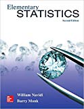
Elementary Statistics 2nd Edition
2nd Edition
ISBN: 9781259724275
Author: William Navidi, Barry Monk
Publisher: McGraw-Hill Education
expand_more
expand_more
format_list_bulleted
Concept explainers
Question
Chapter 2.3, Problem 33E
(a)
To determine
To explain whether the given statement is true or false.
(b)
To determine
Th explain whether the amount is increases from 2010 to 2012.
(c)
To determine
To explain whether the given statement is true or false.
(d)
To determine
To explain whether the given statement is true or false.
Expert Solution & Answer
Want to see the full answer?
Check out a sample textbook solution
Students have asked these similar questions
Use the accompanying Grade Point Averages data to find 80%,85%, and 99%confidence intervals for the mean GPA.
view the Grade Point Averages data.
Gender College GPAFemale Arts and Sciences 3.21Male Engineering 3.87Female Health Science 3.85Male Engineering 3.20Female Nursing 3.40Male Engineering 3.01Female Nursing 3.48Female Nursing 3.26Female Arts and Sciences 3.50Male Engineering 3.00Female Arts and Sciences 3.13Female Nursing 3.34Female Nursing 3.67Female Education 3.45Female Engineering 3.17Female Health Science 3.28Female Nursing 3.25Male Engineering 3.72Female Arts and Sciences 2.68Female Nursing 3.40Female Health Science 3.76Female Arts and Sciences 3.72Female Education 3.44Female Arts and Sciences 3.61Female Education 3.29Female Nursing 3.20Female Education 3.80Female Business 3.26Male…
Business Discuss
Could you please answer this question using excel. For 1a) I got 84.75 and for part 1b) I got 85.33 and was wondering if you could check if my answers were correct. Thanks
Chapter 2 Solutions
Elementary Statistics 2nd Edition
Ch. 2.1 - In Exercises 5-8, fill in each blank with the...Ch. 2.1 - In Exercises 5-8, fill in each blank with the...Ch. 2.1 - In Exercises 5-8, fill in each blank with the...Ch. 2.1 - In Exercises 5-8, fill in each blank with the...Ch. 2.1 - In Exercises 9—12, determine whether the...Ch. 2.1 - In Exercises 9—12, determine whether the...Ch. 2.1 - In Exercises 9—12, determine whether the...Ch. 2.1 - In Exercises 9—12, determine whether the...Ch. 2.1 - The following bar graph presents the average...Ch. 2.1 - The most common blood typing system divides human...
Ch. 2.1 - Following is a pie chart that presents the...Ch. 2.1 - Prob. 16ECh. 2.1 - Food sources: The following side-by-side bar graph...Ch. 2.1 - Prob. 18ECh. 2.1 - Prob. 19ECh. 2.1 - Popular video games: The following frequency...Ch. 2.1 - More iPods: Using the data in exercise 19:...Ch. 2.1 - Prob. 22ECh. 2.1 - Prob. 23ECh. 2.1 - World population: Following are the populations of...Ch. 2.1 - Ages of video garners: The Nielsen Company...Ch. 2.1 - How secure is your job? In a survey, employed...Ch. 2.1 - Back up your data: In a survey commissioned by the...Ch. 2.1 - Education levels: The following frequency...Ch. 2.1 - Music sales: The following frequency distribution...Ch. 2.1 - Bought a new car lately? The following table...Ch. 2.1 - Instagram followers: The following frequency...Ch. 2.1 - Smartphones: The following table present the...Ch. 2.1 - Smartphone sale: The following table presents the...Ch. 2.1 - Happy Halloween: The following table presents...Ch. 2.1 - Native languages: The following frequency...Ch. 2.2 - Prob. 5ECh. 2.2 - In Exercises 5—8, fill in each blank with the...Ch. 2.2 - In Exercises 5—8, fill in each blank with the...Ch. 2.2 - In Exercises 5—8, fill in each blank with the...Ch. 2.2 - In Exercises 9—12, determine whether the...Ch. 2.2 - In Exercises 9—12, determine whether the...Ch. 2.2 - In Exercises 9—12, determine whether the...Ch. 2.2 - In Exercises 9—12, determine whether the...Ch. 2.2 - In Exercises 13—16, classify the histogram as...Ch. 2.2 - In Exercises 13—16, classify the histogram as...Ch. 2.2 - In Exercises 13—16, classify the histogram as...Ch. 2.2 - In Exercises 13—16, classify the histogram as...Ch. 2.2 - In Exercises 17 and 18, classify the histogram as...Ch. 2.2 - In Exercises 17 and 18, classify the histogram as...Ch. 2.2 - Student heights: The following frequency histogram...Ch. 2.2 - Trained rats: Forty rats were trained to run a...Ch. 2.2 - Prob. 21ECh. 2.2 - Prob. 22ECh. 2.2 - Prob. 23ECh. 2.2 - Prob. 24ECh. 2.2 - Batting average: The following frequency...Ch. 2.2 - Batting average: The following frequency...Ch. 2.2 - Time spent playing video games: A sample of 200...Ch. 2.2 - Murder, she wrote: The following frequency...Ch. 2.2 - BMW prices: The following table presents the...Ch. 2.2 - Geysers: The geyser Old Faithful in Yellowstone...Ch. 2.2 - Hail to the chief: There have been 58 presidential...Ch. 2.2 - Internet radio: The following table presents the...Ch. 2.2 - Brothers and sisters: Thirty students in a...Ch. 2.2 - Cough, cough: The following table presents the...Ch. 2.2 - Prob. 35ECh. 2.2 - Frequency polygon: Using the data in Exercise 26:...Ch. 2.2 - Frequency polygon: Using data in Exercise 27:...Ch. 2.2 - Prob. 38ECh. 2.2 - Ogive: Using the data in Exercise 25 Compute the...Ch. 2.2 - Ogive: Using the data in Exercise 26: Compute the...Ch. 2.2 - Ogive: Using the data in Exercise 27: Compute the...Ch. 2.2 - Prob. 42ECh. 2.2 - Prob. 43ECh. 2.2 - Prob. 44ECh. 2.2 - Prob. 45ECh. 2.2 - Prob. 46ECh. 2.2 - Prob. 47ECh. 2.2 - Prob. 48ECh. 2.3 - In Exercises 3—6, fill in each blank with the...Ch. 2.3 - In Exercises 3—6, fill in each blank with the...Ch. 2.3 - In Exercises 3—6, fill in each blank with the...Ch. 2.3 - In Exercises 3—6, fill in each blank with the...Ch. 2.3 - Prob. 7ECh. 2.3 - In Exercises 7—10, determine whether the...Ch. 2.3 - In Exercises 7—10, determine whether the...Ch. 2.3 - In Exercises 7—10, determine whether the...Ch. 2.3 - Construct a stem-and-leaf plot for the following...Ch. 2.3 - Construct a stem-and-leaf plot for the following...Ch. 2.3 - List the data in the following stem-and-leaf plot....Ch. 2.3 - List the data in the following stein-and-leaf...Ch. 2.3 - Construct a dotplot for the data in Exercise 11.Ch. 2.3 - Prob. 16ECh. 2.3 - BMW prices: The following table presents the...Ch. 2.3 - Hows the weather? The following table presents the...Ch. 2.3 - Air pollution: The following table presents...Ch. 2.3 - Technology salaries: The following table presents...Ch. 2.3 - Tennis and golf: Following are the ages of the...Ch. 2.3 - Pass the popcorn: Following are the running times...Ch. 2.3 - More weather: Construct a dotplot for the data in...Ch. 2.3 - Prob. 24ECh. 2.3 - Prob. 25ECh. 2.3 - Prob. 26ECh. 2.3 - Prob. 27ECh. 2.3 - Prob. 28ECh. 2.3 - Prob. 29ECh. 2.3 - Prob. 30ECh. 2.3 - Prob. 31ECh. 2.3 - Prob. 32ECh. 2.3 - Prob. 33ECh. 2.3 - Article ice sheet: the following table presents...Ch. 2.3 - Prob. 35ECh. 2.4 - In Exercises 3 and 4, fill in each blank with the...Ch. 2.4 - In Exercises 3 and 4, fill in each blank with the...Ch. 2.4 - CD sales decline: Sales of CDs have been declining...Ch. 2.4 - Prob. 6ECh. 2.4 - Prob. 7ECh. 2.4 - Prob. 8ECh. 2.4 - Prob. 9ECh. 2.4 - Prob. 10ECh. 2.4 - Prob. 11ECh. 2.4 - Age at marriage: Data compiled by the U.S. Census...Ch. 2.4 - College degrees: Both of the following time-series...Ch. 2.4 - Prob. 14ECh. 2.4 - Prob. 15ECh. 2 - Following is the list of letter grades for...Ch. 2 - Prob. 2CQCh. 2 - Construct a frequency bar graph for the data in...Ch. 2 - Prob. 4CQCh. 2 - Prob. 5CQCh. 2 - Prob. 6CQCh. 2 - Prob. 7CQCh. 2 - Prob. 8CQCh. 2 - Prob. 9CQCh. 2 - Prob. 10CQCh. 2 - Following are the prices (in dollars) for a sample...Ch. 2 - Prob. 12CQCh. 2 - Prob. 13CQCh. 2 - Prob. 14CQCh. 2 - Prob. 15CQCh. 2 - Trust your doctor: The General Social Survey...Ch. 2 - Internet browsers: The following relative...Ch. 2 - Prob. 3RECh. 2 - Prob. 4RECh. 2 - Prob. 5RECh. 2 - House freshmen: Newly elected members of the U.S....Ch. 2 - More freshmen: For the data in Exercise 6:...Ch. 2 - Royalty: Following are the ages at death for all...Ch. 2 - Prob. 9RECh. 2 - Prob. 10RECh. 2 - Prob. 11RECh. 2 - Prob. 12RECh. 2 - Prob. 13RECh. 2 - Prob. 14RECh. 2 - Falling birth rate: The following time-series...Ch. 2 - Explain why the frequency bar graph and the...Ch. 2 - Prob. 2WAICh. 2 - Prob. 3WAICh. 2 - Prob. 4WAICh. 2 - Prob. 5WAICh. 2 - In the chapter introduction, we presented gas...Ch. 2 - In the chapter introduction, we presented gas...Ch. 2 - In the chapter introduction, we presented gas...Ch. 2 - Prob. 4CSCh. 2 - In the chapter introduction, we presented gas...Ch. 2 - Prob. 6CSCh. 2 - In the chapter introduction, we presented gas...Ch. 2 - Prob. 8CSCh. 2 - In the chapter introduction, we presented gas...
Knowledge Booster
Learn more about
Need a deep-dive on the concept behind this application? Look no further. Learn more about this topic, statistics and related others by exploring similar questions and additional content below.Similar questions
- What is one sample T-test? Give an example of business application of this test? What is Two-Sample T-Test. Give an example of business application of this test? .What is paired T-test. Give an example of business application of this test? What is one way ANOVA test. Give an example of business application of this test? 1. One Sample T-Test: Determine whether the average satisfaction rating of customers for a product is significantly different from a hypothetical mean of 75. (Hints: The null can be about maintaining status-quo or no difference; If your alternative hypothesis is non-directional (e.g., μ≠75), you should use the two-tailed p-value from excel file to make a decision about rejecting or not rejecting null. If alternative is directional (e.g., μ < 75), you should use the lower-tailed p-value. For alternative hypothesis μ > 75, you should use the upper-tailed p-value.) H0 = H1= Conclusion: The p value from one sample t-test is _______. Since the two-tailed p-value…arrow_forwardUsing the accompanying Accounting Professionals data to answer the following questions. a. Find and interpret a 90% confidence interval for the mean years of service. b. Find and interpret a 90% confidence interval for the proportion of employees who have a graduate degree. view the Accounting Professionals data. Employee Years of Service Graduate Degree?1 26 Y2 8 N3 10 N4 6 N5 23 N6 5 N7 8 Y8 5 N9 26 N10 14 Y11 10 N12 8 Y13 7 Y14 27 N15 16 Y16 17 N17 21 N18 9 Y19 9 N20 9 N Question content area bottom Part 1 a. A 90% confidence interval for the mean years of service is (Use ascending order. Round to two decimal places as needed.)arrow_forwardIf, based on a sample size of 900,a political candidate finds that 509people would vote for him in a two-person race, what is the 95%confidence interval for his expected proportion of the vote? Would he be confident of winning based on this poll? Question content area bottom Part 1 A 9595% confidence interval for his expected proportion of the vote is (Use ascending order. Round to four decimal places as needed.)arrow_forward
- Questions An insurance company's cumulative incurred claims for the last 5 accident years are given in the following table: Development Year Accident Year 0 2018 1 2 3 4 245 267 274 289 292 2019 255 276 288 294 2020 265 283 292 2021 263 278 2022 271 It can be assumed that claims are fully run off after 4 years. The premiums received for each year are: Accident Year Premium 2018 306 2019 312 2020 318 2021 326 2022 330 You do not need to make any allowance for inflation. 1. (a) Calculate the reserve at the end of 2022 using the basic chain ladder method. (b) Calculate the reserve at the end of 2022 using the Bornhuetter-Ferguson method. 2. Comment on the differences in the reserves produced by the methods in Part 1.arrow_forwardA population that is uniformly distributed between a=0and b=10 is given in sample sizes 50( ), 100( ), 250( ), and 500( ). Find the sample mean and the sample standard deviations for the given data. Compare your results to the average of means for a sample of size 10, and use the empirical rules to analyze the sampling error. For each sample, also find the standard error of the mean using formula given below. Standard Error of the Mean =sigma/Root Complete the following table with the results from the sampling experiment. (Round to four decimal places as needed.) Sample Size Average of 8 Sample Means Standard Deviation of 8 Sample Means Standard Error 50 100 250 500arrow_forwardA survey of 250250 young professionals found that two dash thirdstwo-thirds of them use their cell phones primarily for e-mail. Can you conclude statistically that the population proportion who use cell phones primarily for e-mail is less than 0.720.72? Use a 95% confidence interval. Question content area bottom Part 1 The 95% confidence interval is left bracket nothing comma nothing right bracket0.60820.6082, 0.72510.7251. As 0.720.72 is within the limits of the confidence interval, we cannot conclude that the population proportion is less than 0.720.72. (Use ascending order. Round to four decimal places as needed.)arrow_forward
- I need help with this problem and an explanation of the solution for the image described below. (Statistics: Engineering Probabilities)arrow_forwardA survey of 250 young professionals found that two-thirds of them use their cell phones primarily for e-mail. Can you conclude statistically that the population proportion who use cell phones primarily for e-mail is less than 0.72? Use a 95% confidence interval. Question content area bottom Part 1 The 95% confidence interval is [ ], [ ] As 0.72 is ▼ above the upper limit within the limits below the lower limit of the confidence interval, we ▼ can cannot conclude that the population proportion is less than 0.72. (Use ascending order. Round to four decimal places as needed.)arrow_forwardI need help with this problem and an explanation of the solution for the image described below. (Statistics: Engineering Probabilities)arrow_forward
- I need help with this problem and an explanation of the solution for the image described below. (Statistics: Engineering Probabilities)arrow_forwardI need help with this problem and an explanation of the solution for the image described below. (Statistics: Engineering Probabilities)arrow_forwardQuestions An insurance company's cumulative incurred claims for the last 5 accident years are given in the following table: Development Year Accident Year 0 2018 1 2 3 4 245 267 274 289 292 2019 255 276 288 294 2020 265 283 292 2021 263 278 2022 271 It can be assumed that claims are fully run off after 4 years. The premiums received for each year are: Accident Year Premium 2018 306 2019 312 2020 318 2021 326 2022 330 You do not need to make any allowance for inflation. 1. (a) Calculate the reserve at the end of 2022 using the basic chain ladder method. (b) Calculate the reserve at the end of 2022 using the Bornhuetter-Ferguson method. 2. Comment on the differences in the reserves produced by the methods in Part 1.arrow_forward
arrow_back_ios
SEE MORE QUESTIONS
arrow_forward_ios
Recommended textbooks for you
 Glencoe Algebra 1, Student Edition, 9780079039897...AlgebraISBN:9780079039897Author:CarterPublisher:McGraw Hill
 Trigonometry (MindTap Course List)TrigonometryISBN:9781337278461Author:Ron LarsonPublisher:Cengage Learning
 Elementary AlgebraAlgebraISBN:9780998625713Author:Lynn Marecek, MaryAnne Anthony-SmithPublisher:OpenStax - Rice University

 Algebra and Trigonometry (MindTap Course List)AlgebraISBN:9781305071742Author:James Stewart, Lothar Redlin, Saleem WatsonPublisher:Cengage Learning

Glencoe Algebra 1, Student Edition, 9780079039897...
Algebra
ISBN:9780079039897
Author:Carter
Publisher:McGraw Hill


Trigonometry (MindTap Course List)
Trigonometry
ISBN:9781337278461
Author:Ron Larson
Publisher:Cengage Learning

Elementary Algebra
Algebra
ISBN:9780998625713
Author:Lynn Marecek, MaryAnne Anthony-Smith
Publisher:OpenStax - Rice University


Algebra and Trigonometry (MindTap Course List)
Algebra
ISBN:9781305071742
Author:James Stewart, Lothar Redlin, Saleem Watson
Publisher:Cengage Learning
Mod-01 Lec-01 Discrete probability distributions (Part 1); Author: nptelhrd;https://www.youtube.com/watch?v=6x1pL9Yov1k;License: Standard YouTube License, CC-BY
Discrete Probability Distributions; Author: Learn Something;https://www.youtube.com/watch?v=m9U4UelWLFs;License: Standard YouTube License, CC-BY
Probability Distribution Functions (PMF, PDF, CDF); Author: zedstatistics;https://www.youtube.com/watch?v=YXLVjCKVP7U;License: Standard YouTube License, CC-BY
Discrete Distributions: Binomial, Poisson and Hypergeometric | Statistics for Data Science; Author: Dr. Bharatendra Rai;https://www.youtube.com/watch?v=lHhyy4JMigg;License: Standard Youtube License