
Introduction to Statistics and Data Analysis
5th Edition
ISBN: 9781305115347
Author: Roxy Peck; Chris Olsen; Jay L. Devore
Publisher: Brooks Cole
expand_more
expand_more
format_list_bulleted
Concept explainers
Videos
Textbook Question
Chapter 14.3, Problem 40E
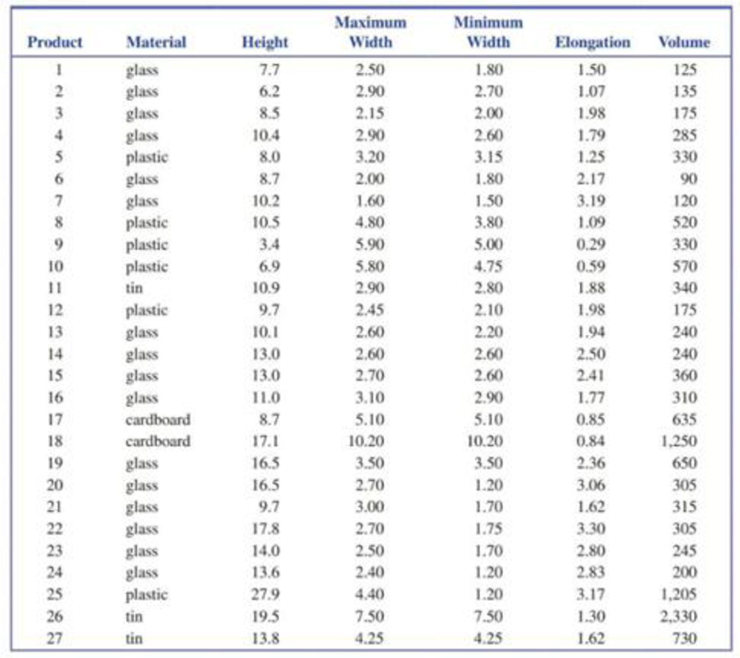
The article first introduced in Exercise 14.28 of Section 14.2 in the textbook gave data on the dimensions of 27 representative food products. Use the multiple regression model fit in Exercise 14.28.
- a. Could any of the variables be eliminated from the estimated regression equation for predicting volume?
- b. Predict the volume of a package with a minimum width of 2.5 cm, a maximum width of 3.0 cm, and an elongation of 1.55.
- c. Calculate a 95% prediction interval for the volume of a package with a minimum width of 2.5 cm, a maximum width of 3.0 cm, and an elongation of 1.55.
14.28 This exercise requires the use of a statistical software package. The article “Vital Dimensions in Volume Perception: Can the Eye Fool the Stomach?” (Journal of Marketing Research [1999]: 313-326) gave the data, shown in the table below, on dimensions of 27 representative food products.
- a. Fit a multiple regression model for predicting the volume (in ml) of a package based on its minimum width, maximum width, and elongation score.
- b. Why should we consider adjusted R: instead of R: when evaluating this model?
- c. Carry out a model utility F test.
Table for exercise 14.28
Expert Solution & Answer
Want to see the full answer?
Check out a sample textbook solution
Students have asked these similar questions
The following are suggested designs for group sequential studies. Using PROCSEQDESIGN, provide the following for the design O’Brien Fleming and Pocock.• The critical boundary values for each analysis of the data• The expected sample sizes at each interim analysisAssume the standardized Z score method for calculating boundaries.Investigators are evaluating the success rate of a novel drug for treating a certain type ofbacterial wound infection. Since no existing treatment exists, they have planned a one-armstudy. They wish to test whether the success rate of the drug is better than 50%, whichthey have defined as the null success rate. Preliminary testing has estimated the successrate of the drug at 55%. The investigators are eager to get the drug into production andwould like to plan for 9 interim analyses (10 analyzes in total) of the data. Assume thesignificance level is 5% and power is 90%.Besides, draw a combined boundary plot (OBF, POC, and HP)
Please provide the solution for the attached image in detailed.
20 km, because
GISS
Worksheet 10
Jesse runs a small business selling and delivering mealie meal to the spaza shops.
He charges a fixed rate of R80, 00 for delivery and then R15, 50 for each packet of
mealle meal he delivers. The table below helps him to calculate what to charge
his customers.
10
20
30
40
50
Packets of mealie
meal (m)
Total costs in Rands
80
235
390
545
700
855
(c)
10.1.
Define the following terms:
10.1.1. Independent Variables
10.1.2. Dependent Variables
10.2.
10.3.
10.4.
10.5.
Determine the independent and dependent variables.
Are the variables in this scenario discrete or continuous values? Explain
What shape do you expect the graph to be? Why?
Draw a graph on the graph provided to represent the information in the
table above.
TOTAL COST OF PACKETS OF MEALIE MEAL
900
800
700
600
COST (R)
500
400
300
200
100
0
10
20
30
40
60
NUMBER OF PACKETS OF MEALIE MEAL
Chapter 14 Solutions
Introduction to Statistics and Data Analysis
Ch. 14.1 - Prob. 1ECh. 14.1 - The authors of the paper Weight-Bearing Activity...Ch. 14.1 - Prob. 3ECh. 14.1 - Prob. 4ECh. 14.1 - Prob. 5ECh. 14.1 - Prob. 6ECh. 14.1 - Prob. 7ECh. 14.1 - Prob. 8ECh. 14.1 - Prob. 9ECh. 14.1 - The relationship between yield of maize (a type of...
Ch. 14.1 - Prob. 11ECh. 14.1 - A manufacturer of wood stoves collected data on y...Ch. 14.1 - Prob. 13ECh. 14.1 - Prob. 14ECh. 14.1 - Prob. 15ECh. 14.2 - Prob. 16ECh. 14.2 - State as much information as you can about the...Ch. 14.2 - Prob. 18ECh. 14.2 - Prob. 19ECh. 14.2 - Prob. 20ECh. 14.2 - The ability of ecologists to identify regions of...Ch. 14.2 - Prob. 22ECh. 14.2 - Prob. 23ECh. 14.2 - Prob. 24ECh. 14.2 - Prob. 25ECh. 14.2 - Prob. 26ECh. 14.2 - This exercise requires the use of a statistical...Ch. 14.2 - Prob. 28ECh. 14.2 - The article The Undrained Strength of Some Thawed...Ch. 14.2 - Prob. 30ECh. 14.2 - Prob. 31ECh. 14.2 - Prob. 32ECh. 14.2 - Prob. 33ECh. 14.2 - This exercise requires the use of a statistical...Ch. 14.2 - This exercise requires the use of a statistical...Ch. 14.3 - Prob. 36ECh. 14.3 - Prob. 37ECh. 14.3 - Prob. 38ECh. 14.3 - Prob. 39ECh. 14.3 - The article first introduced in Exercise 14.28 of...Ch. 14.3 - Data from a random sample of 107 students taking a...Ch. 14.3 - Benevolence payments are monies collected by a...Ch. 14.3 - Prob. 43ECh. 14.3 - Prob. 44ECh. 14.3 - Prob. 45ECh. 14.3 - Prob. 46ECh. 14.3 - Exercise 14.26 gave data on fish weight, length,...Ch. 14.3 - Prob. 48ECh. 14.3 - Prob. 49ECh. 14.3 - Prob. 50ECh. 14.4 - Prob. 51ECh. 14.4 - Prob. 52ECh. 14.4 - The article The Analysis and Selection of...Ch. 14.4 - Prob. 54ECh. 14.4 - Prob. 55ECh. 14.4 - Prob. 57ECh. 14.4 - Prob. 58ECh. 14.4 - Prob. 59ECh. 14.4 - Prob. 60ECh. 14.4 - This exercise requires use of a statistical...Ch. 14.4 - Prob. 62ECh. 14 - Prob. 63CRCh. 14 - Prob. 64CRCh. 14 - The accompanying data on y = Glucose concentration...Ch. 14 - Much interest in management circles has focused on...Ch. 14 - Prob. 67CRCh. 14 - Prob. 68CRCh. 14 - Prob. 69CRCh. 14 - A study of pregnant grey seals resulted in n = 25...Ch. 14 - Prob. 71CRCh. 14 - Prob. 72CRCh. 14 - This exercise requires the use of a statistical...
Knowledge Booster


Learn more about
Need a deep-dive on the concept behind this application? Look no further. Learn more about this topic, statistics and related others by exploring similar questions and additional content below.Similar questions
- Let X be a random variable with support SX = {−3, 0.5, 3, −2.5, 3.5}. Part ofits probability mass function (PMF) is given bypX(−3) = 0.15, pX(−2.5) = 0.3, pX(3) = 0.2, pX(3.5) = 0.15.(a) Find pX(0.5).(b) Find the cumulative distribution function (CDF), FX(x), of X.1(c) Sketch the graph of FX(x).arrow_forwardA well-known company predominantly makes flat pack furniture for students. Variability with the automated machinery means the wood components are cut with a standard deviation in length of 0.45 mm. After they are cut the components are measured. If their length is more than 1.2 mm from the required length, the components are rejected. a) Calculate the percentage of components that get rejected. b) In a manufacturing run of 1000 units, how many are expected to be rejected? c) The company wishes to install more accurate equipment in order to reduce the rejection rate by one-half, using the same ±1.2mm rejection criterion. Calculate the maximum acceptable standard deviation of the new process.arrow_forward5. Let X and Y be independent random variables and let the superscripts denote symmetrization (recall Sect. 3.6). Show that (X + Y) X+ys.arrow_forward
- 8. Suppose that the moments of the random variable X are constant, that is, suppose that EX" =c for all n ≥ 1, for some constant c. Find the distribution of X.arrow_forward9. The concentration function of a random variable X is defined as Qx(h) = sup P(x ≤ X ≤x+h), h>0. Show that, if X and Y are independent random variables, then Qx+y (h) min{Qx(h). Qr (h)).arrow_forward10. Prove that, if (t)=1+0(12) as asf->> O is a characteristic function, then p = 1.arrow_forward
- 9. The concentration function of a random variable X is defined as Qx(h) sup P(x ≤x≤x+h), h>0. (b) Is it true that Qx(ah) =aQx (h)?arrow_forward3. Let X1, X2,..., X, be independent, Exp(1)-distributed random variables, and set V₁₁ = max Xk and W₁ = X₁+x+x+ Isk≤narrow_forward7. Consider the function (t)=(1+|t|)e, ER. (a) Prove that is a characteristic function. (b) Prove that the corresponding distribution is absolutely continuous. (c) Prove, departing from itself, that the distribution has finite mean and variance. (d) Prove, without computation, that the mean equals 0. (e) Compute the density.arrow_forward
- 1. Show, by using characteristic, or moment generating functions, that if fx(x) = ½ex, -∞0 < x < ∞, then XY₁ - Y2, where Y₁ and Y2 are independent, exponentially distributed random variables.arrow_forward1. Show, by using characteristic, or moment generating functions, that if 1 fx(x): x) = ½exarrow_forward1990) 02-02 50% mesob berceus +7 What's the probability of getting more than 1 head on 10 flips of a fair coin?arrow_forward
arrow_back_ios
SEE MORE QUESTIONS
arrow_forward_ios
Recommended textbooks for you
 Functions and Change: A Modeling Approach to Coll...AlgebraISBN:9781337111348Author:Bruce Crauder, Benny Evans, Alan NoellPublisher:Cengage Learning
 Algebra & Trigonometry with Analytic GeometryAlgebraISBN:9781133382119Author:SwokowskiPublisher:Cengage
 College AlgebraAlgebraISBN:9781305115545Author:James Stewart, Lothar Redlin, Saleem WatsonPublisher:Cengage Learning
 Algebra and Trigonometry (MindTap Course List)AlgebraISBN:9781305071742Author:James Stewart, Lothar Redlin, Saleem WatsonPublisher:Cengage Learning
 Linear Algebra: A Modern IntroductionAlgebraISBN:9781285463247Author:David PoolePublisher:Cengage Learning
Functions and Change: A Modeling Approach to Coll...
Algebra
ISBN:9781337111348
Author:Bruce Crauder, Benny Evans, Alan Noell
Publisher:Cengage Learning
Algebra & Trigonometry with Analytic Geometry
Algebra
ISBN:9781133382119
Author:Swokowski
Publisher:Cengage
College Algebra
Algebra
ISBN:9781305115545
Author:James Stewart, Lothar Redlin, Saleem Watson
Publisher:Cengage Learning
Algebra and Trigonometry (MindTap Course List)
Algebra
ISBN:9781305071742
Author:James Stewart, Lothar Redlin, Saleem Watson
Publisher:Cengage Learning
Linear Algebra: A Modern Introduction
Algebra
ISBN:9781285463247
Author:David Poole
Publisher:Cengage Learning
Correlation Vs Regression: Difference Between them with definition & Comparison Chart; Author: Key Differences;https://www.youtube.com/watch?v=Ou2QGSJVd0U;License: Standard YouTube License, CC-BY
Correlation and Regression: Concepts with Illustrative examples; Author: LEARN & APPLY : Lean and Six Sigma;https://www.youtube.com/watch?v=xTpHD5WLuoA;License: Standard YouTube License, CC-BY