
Concept explainers
Videos
Find the values of k, which correspond to the useful model at the 0.05 level of significance.
Explain the large value of
Answer to Problem 32E
The values of k less than 9 corresponds to the useful model at the 0.05 level of significance.
Explanation of Solution
Calculation:
It is given that the
Test statistic:
Where, n is the sample size and k is the number of variables in the model.
The value of F test statistic is calculated as follows:
For
The value of F test statistic is calculated as follows:
P-value:
Software procedure:
Step-by-step procedure to find the P-value using the MINITAB software:
- Choose Graph >
Probability Distribution Plot choose View Probability > OK. - From Distribution, choose ‘F’ distribution.
- Enter the Numerator df as 1 and Denominator df as 13.
- Click the Shaded Area tab.
- Choose Probability Value and Right Tail for the region of the curve to shade.
- Enter the Probability value as 0.05.
- Click OK.
Output obtained using the MINITAB software is represented as follows:
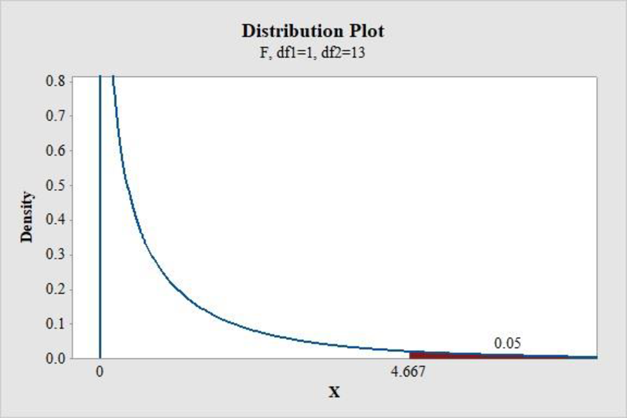
From the MINITAB output, the critical value is 4.667.
Conclusion:
If the F test statistic value is greater than the critical value, then reject the null hypothesis.
Therefore, the F test statistic of 117 is greater than the critical value of 4.667.
Hence, reject the null hypothesis.
Thus, there is convincing evidence that the model is useful.
For
The value of F test statistic is calculated as follows:
P-value:
Software procedure:
Step-by-step procedure to find the P-value using the MINITAB software:
- Choose Graph > Probability Distribution Plot choose View Probability > OK.
- From Distribution, choose ‘F’ distribution.
- Enter the Numerator df as 2 and Denominator df as 12.
- Click the Shaded Area tab.
- Choose Probability Value and Right Tail for the region of the curve to shade.
- Enter the Probability value as 0.05.
- Click OK.
Output obtained using the MINITAB software is represented as follows:
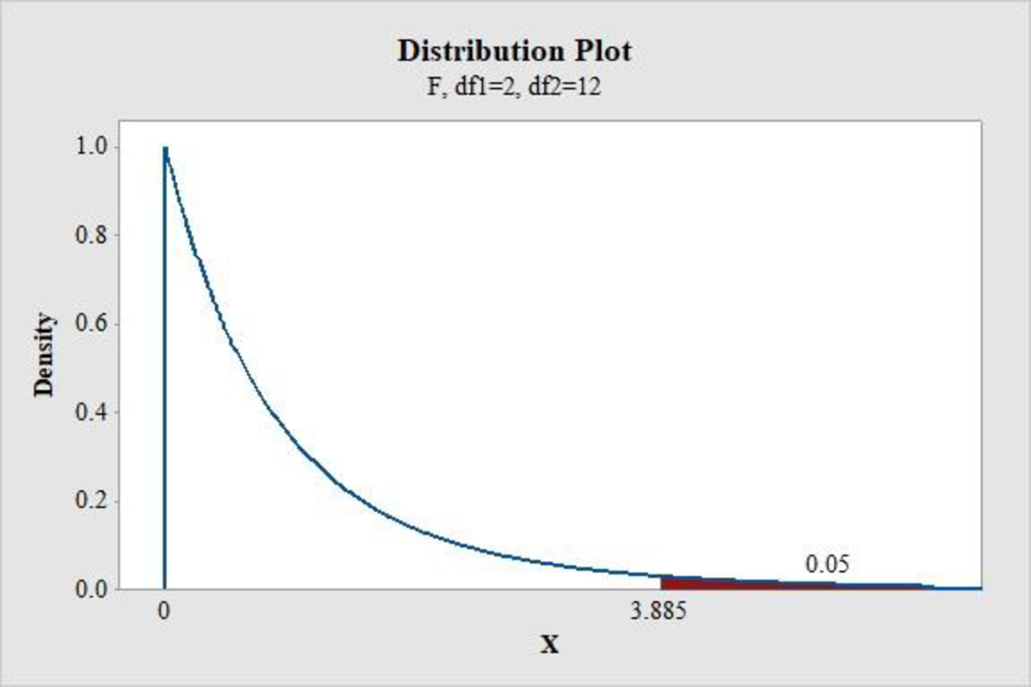
From the MINITAB output, the critical value is 3.885.
Conclusion:
If the F test statistic value is greater than the critical value, then reject the null hypothesis.
Therefore, the F test statistic of 54 is greater than the critical value of 3.885.
Hence, reject the null hypothesis.
Thus, there is convincing evidence that the model is useful.
For
The value of F test statistic is calculated as follows:
P-value:
Software procedure:
Step-by-step procedure to find the P-value using the MINITAB software:
- Choose Graph > Probability Distribution Plot choose View Probability > OK.
- From Distribution, choose ‘F’ distribution.
- Enter the Numerator df as 3 and Denominator df as 11.
- Click the Shaded Area tab.
- Choose Probability Value and Right Tail for the region of the curve to shade.
- Enter the Probability value as 0.05.
- Click OK.
Output obtained using the MINITAB software is represented as follows:
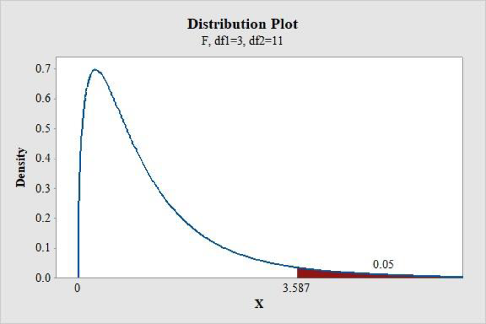
From the MINITAB output, the critical value is 3.587.
Conclusion:
If the F test statistic value is greater than the critical value, then reject the null hypothesis.
Therefore, the F test statistic of 33 is greater than the critical value of 3.587.
Hence, reject the null hypothesis.
Thus, there is convincing evidence that the model is useful.
For
The value of F test statistic is calculated as follows:
P-value:
Software procedure:
Step-by-step procedure to find the P-value using the MINITAB software:
- Choose Graph > Probability Distribution Plot choose View Probability > OK.
- From Distribution, choose ‘F’ distribution.
- Enter the Numerator df as 5 and Denominator df as 9.
- Click the Shaded Area tab.
- Choose Probability Value and Right Tail for the region of the curve to shade.
- Enter the Probability value as 0.05.
- Click OK.
Output obtained using the MINITAB software is represented as follows:
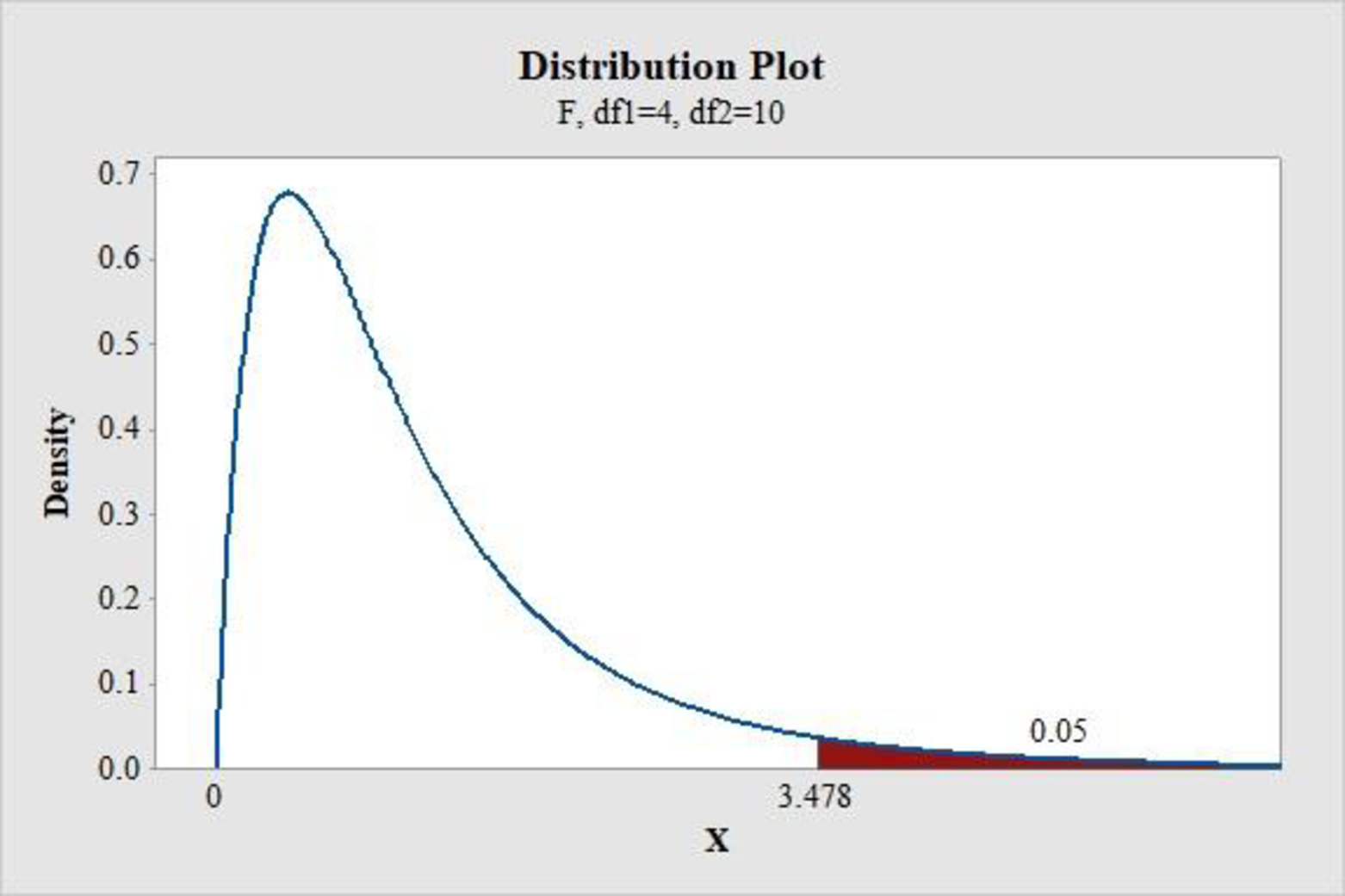
From the MINITAB output, the critical value is 3.478.
Conclusion:
If the F test statistic value is greater than the critical value, then reject the null hypothesis.
Therefore, the F test statistic of 16.2 is greater than the critical value of 3.478.
Hence, reject the null hypothesis.
Thus, there is convincing evidence that the model is useful.
For
The value of F test statistic is calculated as follows:
P-value:
Software procedure:
Step-by-step procedure to find the P-value using the MINITAB software:
- Choose Graph > Probability Distribution Plot choose View Probability > OK.
- From Distribution, choose ‘F’ distribution.
- Enter the Numerator df as 6 and Denominator df as 8.
- Click the Shaded Area tab.
- Choose Probability Value and Right Tail for the region of the curve to shade.
- Enter the Probability value as 0.05.
- Click OK.
Output obtained using the MINITAB software is represented as follows:

From the MINITAB output, the critical value is 3.482.
Conclusion:
If the F test statistic value is greater than the critical value, then reject the null hypothesis.
Therefore, the F test statistic of 12 is greater than the critical value of 3.482.
Hence, reject the null hypothesis.
Thus, there is convincing evidence that the model is useful.
For
The value of F test statistic is calculated as follows:
P-value:
Software procedure:
Step-by-step procedure to find the P-value using the MINITAB software:
- Choose Graph > Probability Distribution Plot choose View Probability > OK.
- From Distribution, choose ‘F’ distribution.
- Enter the Numerator df as 7 and Denominator df as 7.
- Click the Shaded Area tab.
- Choose Probability Value and Right Tail for the region of the curve to shade.
- Enter the Probability value as 0.05.
- Click OK.
Output obtained using the MINITAB software is represented as follows:

From the MINITAB output, the critical value is 3.581.
Conclusion:
If the F test statistic value is greater than the critical value, then reject the null hypothesis.
Therefore, the F test statistic of 9 is greater than the critical value of 3.581.
Hence, reject the null hypothesis.
Thus, there is convincing evidence that the model is useful.
For
The value of F test statistic is calculated as follows:
P-value:
Software procedure:
Step-by-step procedure to find the P-value using the MINITAB software:
- Choose Graph > Probability Distribution Plot choose View Probability > OK.
- From Distribution, choose ‘F’ distribution.
- Enter the Numerator df as 8 and Denominator df as 6.
- Click the Shaded Area tab.
- Choose Probability Value and Right Tail for the region of the curve to shade.
- Enter the Probability value as 0.05.
- Click OK.
Output obtained using the MINITAB software is represented as follows:
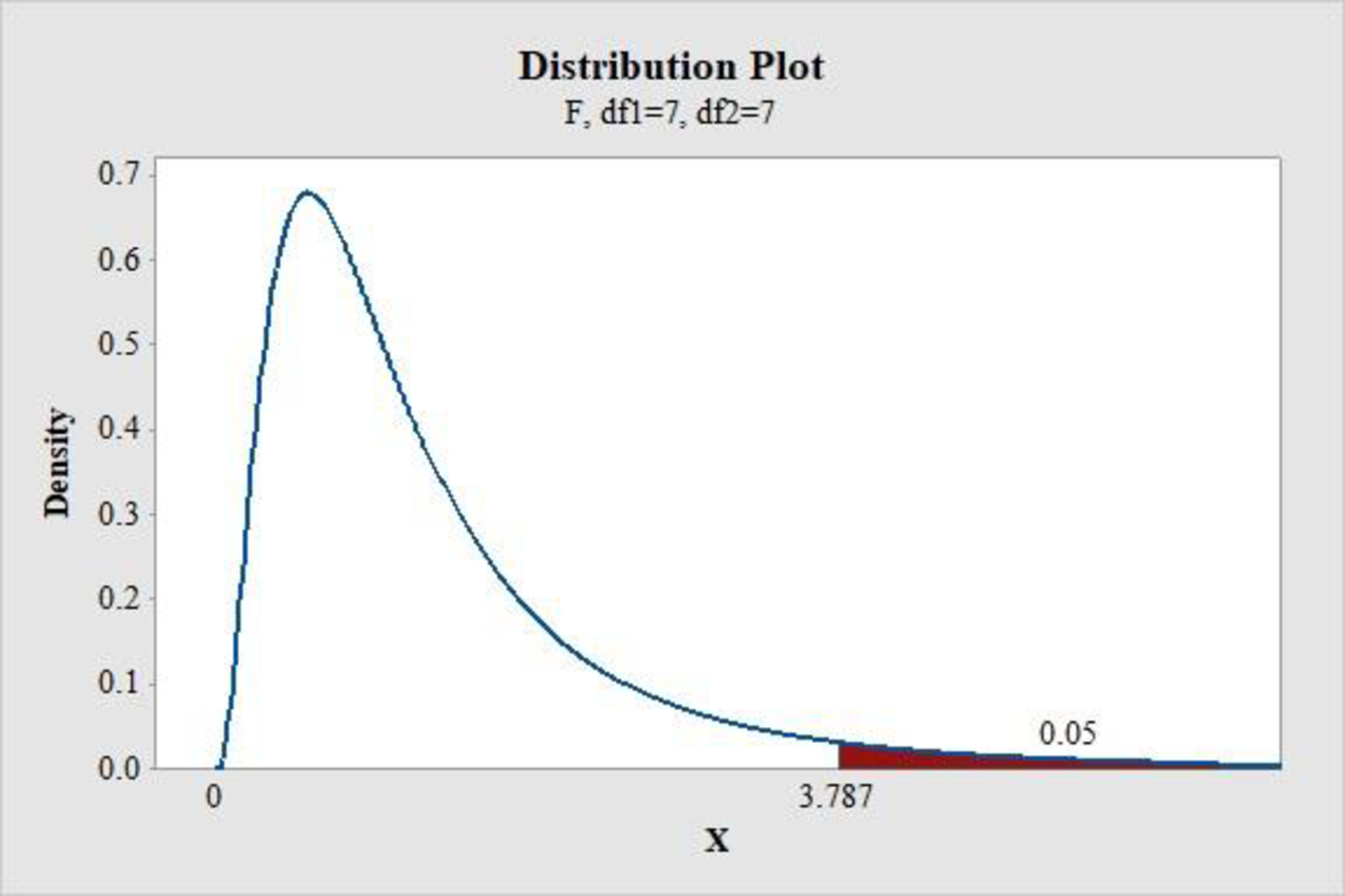
From the MINITAB output, the critical value is 3.787.
Conclusion:
If the F test statistic value is greater than the critical value, then reject the null hypothesis.
Therefore, the F test statistic of 6.75 is greater than the critical value of 3.787.
Hence, reject the null hypothesis.
Thus, there is convincing evidence that the model is useful.
For
The value of F test statistic is calculated as follows:
P-value:
Software procedure:
Step-by-step procedure to find the P-value using the MINITAB software:
- Choose Graph > Probability Distribution Plot choose View Probability > OK.
- From Distribution, choose ‘F’ distribution.
- Enter the Numerator df as 9 and Denominator df as 5.
- Click the Shaded Area tab.
- Choose Probability Value and Right Tail for the region of the curve to shade.
- Enter the Probability value as 0.05.
- Click OK.
Output obtained using the MINITAB software is represented as follows:
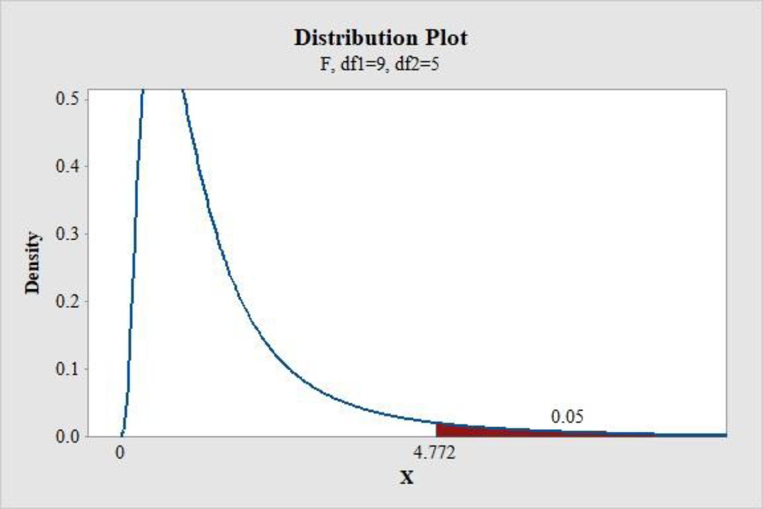
From the MINITAB output, the critical value is 4.772.
Conclusion:
If the F test statistic value is greater than the critical value, then reject the null hypothesis.
Therefore, the F test statistic of 5 is greater than the critical value of 4.772.
Hence, reject the null hypothesis.
Thus, there is convincing evidence that the model is useful.
For
The value of F test statistic is calculated as follows:
P-value:
Software procedure:
Step-by-step procedure to find the P-value using the MINITAB software:
- Choose Graph > Probability Distribution Plot choose View Probability > OK.
- From Distribution, choose ‘F’ distribution.
- Enter the Numerator df as 10 and Denominator df as 4.
- Click the Shaded Area tab.
- Choose Probability Value and Right Tail for the region of the curve to shade.
- Enter the Probability value as 0.05.
- Click OK.
Output obtained using the MINITAB software is represented as follows:
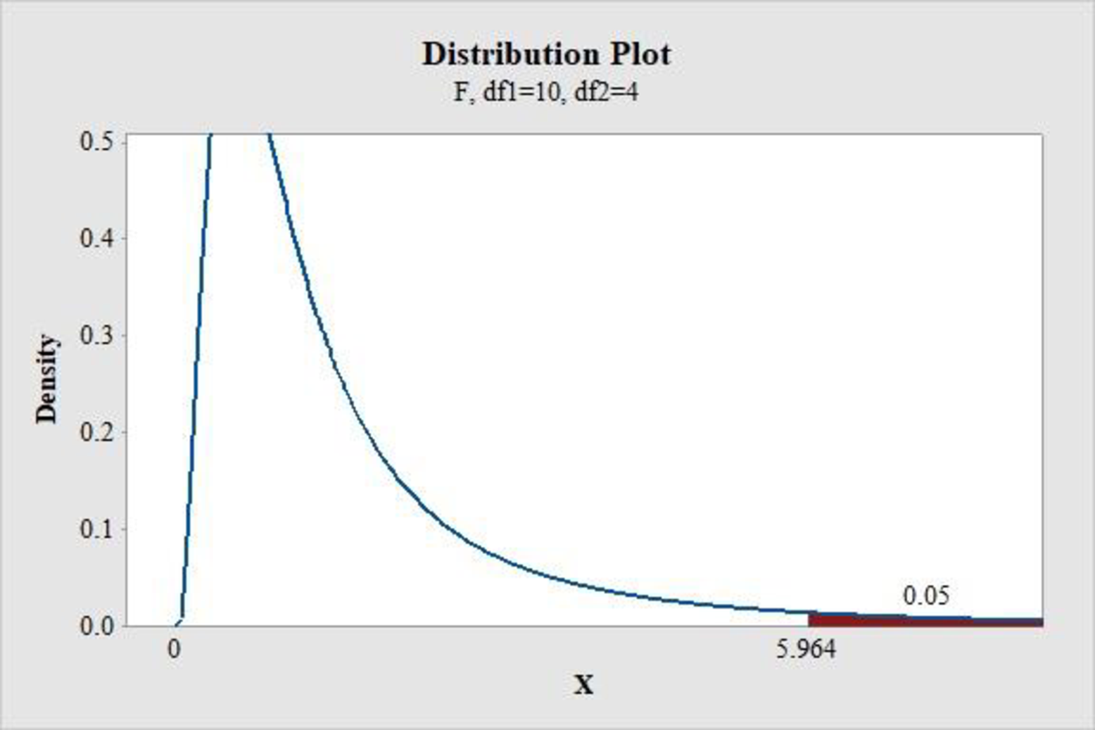
From the MINITAB output, the critical value is 5.964.
Conclusion:
If the F test statistic value is greater than the critical value, then reject the null hypothesis.
Therefore, the F test statistic of 3.6 is less than the critical value of 5.964.
Hence, fail to reject the null hypothesis.
Thus, there is convincing evidence that the model is not useful.
Conclusion:
For the value of k less than 9, there is evidence that the model is useful. For
Want to see more full solutions like this?
Chapter 14 Solutions
Introduction to Statistics and Data Analysis


- a. Find the value of A.b. Find pX(x) and py(y).c. Find pX|y(x|y) and py|X(y|x)d. Are x and y independent? Why or why not?arrow_forwardAnalyze the residuals of a linear regression model and select the best response.Criteria is simple evaluation of possible indications of an exponential model vs. linear model) no, the residual plot does not show a curve yes, the residual plot does not show a curve yes, the residual plot shows a curve no, the residual plot shows a curve I selected: yes, the residual plot shows a curve and it is INCORRECT. Can u help me understand why?arrow_forwardYou have been hired as an intern to run analyses on the data and report the results back to Sarah; the five questions that Sarah needs you to address are given below. please do it step by step on excel Does there appear to be a positive or negative relationship between price and screen size? Use a scatter plot to examine the relationship. Determine and interpret the correlation coefficient between the two variables. In your interpretation, discuss the direction of the relationship (positive, negative, or zero relationship). Also discuss the strength of the relationship. Estimate the relationship between screen size and price using a simple linear regression model and interpret the estimated coefficients. (In your interpretation, tell the dollar amount by which price will change for each unit of increase in screen size). Include the manufacturer dummy variable (Samsung=1, 0 otherwise) and estimate the relationship between screen size, price and manufacturer dummy as a multiple…arrow_forward
- Here is data with as the response variable. x y54.4 19.124.9 99.334.5 9.476.6 0.359.4 4.554.4 0.139.2 56.354 15.773.8 9-156.1 319.2Make a scatter plot of this data. Which point is an outlier? Enter as an ordered pair, e.g., (x,y). (x,y)= Find the regression equation for the data set without the outlier. Enter the equation of the form mx+b rounded to three decimal places. y_wo= Find the regression equation for the data set with the outlier. Enter the equation of the form mx+b rounded to three decimal places. y_w=arrow_forwardYou have been hired as an intern to run analyses on the data and report the results back to Sarah; the five questions that Sarah needs you to address are given below. please do it step by step Does there appear to be a positive or negative relationship between price and screen size? Use a scatter plot to examine the relationship. Determine and interpret the correlation coefficient between the two variables. In your interpretation, discuss the direction of the relationship (positive, negative, or zero relationship). Also discuss the strength of the relationship. Estimate the relationship between screen size and price using a simple linear regression model and interpret the estimated coefficients. (In your interpretation, tell the dollar amount by which price will change for each unit of increase in screen size). Include the manufacturer dummy variable (Samsung=1, 0 otherwise) and estimate the relationship between screen size, price and manufacturer dummy as a multiple linear…arrow_forwardExercises: Find all the whole number solutions of the congruence equation. 1. 3x 8 mod 11 2. 2x+3= 8 mod 12 3. 3x+12= 7 mod 10 4. 4x+6= 5 mod 8 5. 5x+3= 8 mod 12arrow_forward
- Scenario Sales of products by color follow a peculiar, but predictable, pattern that determines how many units will sell in any given year. This pattern is shown below Product Color 1995 1996 1997 Red 28 42 21 1998 23 1999 29 2000 2001 2002 Unit Sales 2003 2004 15 8 4 2 1 2005 2006 discontinued Green 26 39 20 22 28 14 7 4 2 White 43 65 33 36 45 23 12 Brown 58 87 44 48 60 Yellow 37 56 28 31 Black 28 42 21 Orange 19 29 Purple Total 28 42 21 49 68 78 95 123 176 181 164 127 24 179 Questions A) Which color will sell the most units in 2007? B) Which color will sell the most units combined in the 2007 to 2009 period? Please show all your analysis, leave formulas in cells, and specify any assumptions you make.arrow_forwardOne hundred students were surveyed about their preference between dogs and cats. The following two-way table displays data for the sample of students who responded to the survey. Preference Male Female TOTAL Prefers dogs \[36\] \[20\] \[56\] Prefers cats \[10\] \[26\] \[36\] No preference \[2\] \[6\] \[8\] TOTAL \[48\] \[52\] \[100\] problem 1 Find the probability that a randomly selected student prefers dogs.Enter your answer as a fraction or decimal. \[P\left(\text{prefers dogs}\right)=\] Incorrect Check Hide explanation Preference Male Female TOTAL Prefers dogs \[\blueD{36}\] \[\blueD{20}\] \[\blueE{56}\] Prefers cats \[10\] \[26\] \[36\] No preference \[2\] \[6\] \[8\] TOTAL \[48\] \[52\] \[100\] There were \[\blueE{56}\] students in the sample who preferred dogs out of \[100\] total students.arrow_forwardBusiness discussarrow_forward
- You have been hired as an intern to run analyses on the data and report the results back to Sarah; the five questions that Sarah needs you to address are given below. Does there appear to be a positive or negative relationship between price and screen size? Use a scatter plot to examine the relationship. Determine and interpret the correlation coefficient between the two variables. In your interpretation, discuss the direction of the relationship (positive, negative, or zero relationship). Also discuss the strength of the relationship. Estimate the relationship between screen size and price using a simple linear regression model and interpret the estimated coefficients. (In your interpretation, tell the dollar amount by which price will change for each unit of increase in screen size). Include the manufacturer dummy variable (Samsung=1, 0 otherwise) and estimate the relationship between screen size, price and manufacturer dummy as a multiple linear regression model. Interpret the…arrow_forwardDoes there appear to be a positive or negative relationship between price and screen size? Use a scatter plot to examine the relationship. How to take snapshots: if you use a MacBook, press Command+ Shift+4 to take snapshots. If you are using Windows, use the Snipping Tool to take snapshots. Question 1: Determine and interpret the correlation coefficient between the two variables. In your interpretation, discuss the direction of the relationship (positive, negative, or zero relationship). Also discuss the strength of the relationship. Value of correlation coefficient: Direction of the relationship (positive, negative, or zero relationship): Strength of the relationship (strong/moderate/weak): Question 2: Estimate the relationship between screen size and price using a simple linear regression model and interpret the estimated coefficients. In your interpretation, tell the dollar amount by which price will change for each unit of increase in screen size. (The answer for the…arrow_forwardIn this problem, we consider a Brownian motion (W+) t≥0. We consider a stock model (St)t>0 given (under the measure P) by d.St 0.03 St dt + 0.2 St dwt, with So 2. We assume that the interest rate is r = 0.06. The purpose of this problem is to price an option on this stock (which we name cubic put). This option is European-type, with maturity 3 months (i.e. T = 0.25 years), and payoff given by F = (8-5)+ (a) Write the Stochastic Differential Equation satisfied by (St) under the risk-neutral measure Q. (You don't need to prove it, simply give the answer.) (b) Give the price of a regular European put on (St) with maturity 3 months and strike K = 2. (c) Let X = S. Find the Stochastic Differential Equation satisfied by the process (Xt) under the measure Q. (d) Find an explicit expression for X₁ = S3 under measure Q. (e) Using the results above, find the price of the cubic put option mentioned above. (f) Is the price in (e) the same as in question (b)? (Explain why.)arrow_forward
 Glencoe Algebra 1, Student Edition, 9780079039897...AlgebraISBN:9780079039897Author:CarterPublisher:McGraw Hill
 Big Ideas Math A Bridge To Success Algebra 1: Stu...AlgebraISBN:9781680331141Author:HOUGHTON MIFFLIN HARCOURTPublisher:Houghton Mifflin Harcourt
 Holt Mcdougal Larson Pre-algebra: Student Edition...AlgebraISBN:9780547587776Author:HOLT MCDOUGALPublisher:HOLT MCDOUGAL
 Linear Algebra: A Modern IntroductionAlgebraISBN:9781285463247Author:David PoolePublisher:Cengage Learning
 Functions and Change: A Modeling Approach to Coll...AlgebraISBN:9781337111348Author:Bruce Crauder, Benny Evans, Alan NoellPublisher:Cengage Learning
 College AlgebraAlgebraISBN:9781305115545Author:James Stewart, Lothar Redlin, Saleem WatsonPublisher:Cengage Learning