
Concept explainers
Videos
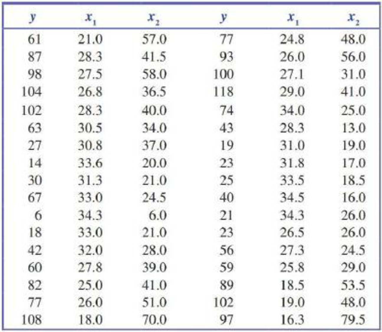
This exercise requires the use of a statistical software package. The cotton aphid poses a threat to cotton crops. The accompanying data on
appeared in the article “Estimation of the Economic Threshold of Infestation for Cotton Aphid” (Mesopotamia Journal of Agriculture [1982]: 71–75). Use the data to find the estimated regression equation and assess the utility of the multiple regression model
Want to see the full answer?
Check out a sample textbook solution
Chapter 14 Solutions
Introduction to Statistics and Data Analysis


- A well-known company predominantly makes flat pack furniture for students. Variability with the automated machinery means the wood components are cut with a standard deviation in length of 0.45 mm. After they are cut the components are measured. If their length is more than 1.2 mm from the required length, the components are rejected. a) Calculate the percentage of components that get rejected. b) In a manufacturing run of 1000 units, how many are expected to be rejected? c) The company wishes to install more accurate equipment in order to reduce the rejection rate by one-half, using the same ±1.2mm rejection criterion. Calculate the maximum acceptable standard deviation of the new process.arrow_forward5. Let X and Y be independent random variables and let the superscripts denote symmetrization (recall Sect. 3.6). Show that (X + Y) X+ys.arrow_forward8. Suppose that the moments of the random variable X are constant, that is, suppose that EX" =c for all n ≥ 1, for some constant c. Find the distribution of X.arrow_forward
- 9. The concentration function of a random variable X is defined as Qx(h) = sup P(x ≤ X ≤x+h), h>0. Show that, if X and Y are independent random variables, then Qx+y (h) min{Qx(h). Qr (h)).arrow_forward10. Prove that, if (t)=1+0(12) as asf->> O is a characteristic function, then p = 1.arrow_forward9. The concentration function of a random variable X is defined as Qx(h) sup P(x ≤x≤x+h), h>0. (b) Is it true that Qx(ah) =aQx (h)?arrow_forward
- 3. Let X1, X2,..., X, be independent, Exp(1)-distributed random variables, and set V₁₁ = max Xk and W₁ = X₁+x+x+ Isk≤narrow_forward7. Consider the function (t)=(1+|t|)e, ER. (a) Prove that is a characteristic function. (b) Prove that the corresponding distribution is absolutely continuous. (c) Prove, departing from itself, that the distribution has finite mean and variance. (d) Prove, without computation, that the mean equals 0. (e) Compute the density.arrow_forward1. Show, by using characteristic, or moment generating functions, that if fx(x) = ½ex, -∞0 < x < ∞, then XY₁ - Y2, where Y₁ and Y2 are independent, exponentially distributed random variables.arrow_forward
- 1. Show, by using characteristic, or moment generating functions, that if 1 fx(x): x) = ½exarrow_forward1990) 02-02 50% mesob berceus +7 What's the probability of getting more than 1 head on 10 flips of a fair coin?arrow_forward9. The concentration function of a random variable X is defined as Qx(h) sup P(x≤x≤x+h), h>0. = x (a) Show that Qx+b(h) = Qx(h).arrow_forward
 MATLAB: An Introduction with ApplicationsStatisticsISBN:9781119256830Author:Amos GilatPublisher:John Wiley & Sons Inc
 Probability and Statistics for Engineering and th...StatisticsISBN:9781305251809Author:Jay L. DevorePublisher:Cengage Learning
 Statistics for The Behavioral Sciences (MindTap C...StatisticsISBN:9781305504912Author:Frederick J Gravetter, Larry B. WallnauPublisher:Cengage Learning
 Elementary Statistics: Picturing the World (7th E...StatisticsISBN:9780134683416Author:Ron Larson, Betsy FarberPublisher:PEARSON
 The Basic Practice of StatisticsStatisticsISBN:9781319042578Author:David S. Moore, William I. Notz, Michael A. FlignerPublisher:W. H. Freeman
 Introduction to the Practice of StatisticsStatisticsISBN:9781319013387Author:David S. Moore, George P. McCabe, Bruce A. CraigPublisher:W. H. Freeman