
Videos
a.
Test whether the given model is useful or not at the 0.05 level of significance.
a.
Answer to Problem 46E
There is convincing evidence that the given model is useful at the 0.05 level of significance.
Explanation of Solution
Calculation:
It is given that the variable y is absorption,
1.
The model is
2.
Null hypothesis:
That is, there is no useful relationship between y and any of the predictors.
3.
Alternative hypothesis:
That is, there is a useful relationship between y and any of the predictors.
4.
Here, the significance level is
5.
Test statistic:
Here, n is the sample size, and k is the number of variables in the model.
6.
Assumptions:
Since there is no availability of original data to check the assumptions, there is a need to assume that the variables are related to the model, and the random deviation is distributed normally with mean 0 and the fixed standard deviation.
7.
Calculation:
From the MINITAB output, the value of
The value of F-test statistic is calculated as follows:
8.
P-value:
Software procedure:
Step-by-step procedure to find the P-value using the MINITAB software:
- Choose Graph > Probability Distribution Plot choose View Probability > OK.
- From Distribution, choose ‘F’ distribution.
- Enter the Numerator df as 2 and Denominator df as 25.
- Click the Shaded Area tab.
- Choose X Value and Right Tail for the region of the curve to shade.
- Enter the X value as 334.722.
- Click OK.
Output obtained using the MINITAB software is represented as follows:
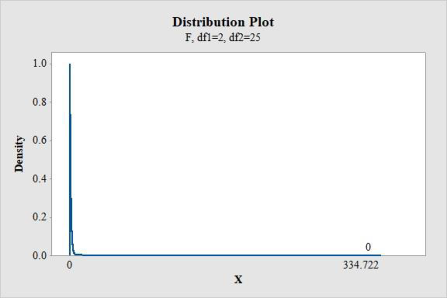
From the MINITAB output, the P-value is 0.
9.
Conclusion:
If the
Therefore, the P-value of 0 is less than the 0.05 level of significance.
Hence, reject the null hypothesis.
Thus, there is convincing evidence that the given model is useful at the 0.05 level of significance.
b.
Calculate a 95% confidence interval for
b.
Answer to Problem 46E
The 95% confidence interval for
Explanation of Solution
Calculation:
Here,
Since there is no availability of original data to check the assumptions, there is a need to assume that the variables are related to the model, and the random deviation is distributed normally with mean 0 and the fixed standard deviation.
The formula for confidence interval for
Where,
Degrees of freedom:
Software procedure:
Step-by-step procedure to find the P-value using the MINITAB software:
- Choose Graph > Probability Distribution Plot choose View Probability > OK.
- From Distribution, choose ‘t’ distribution.
- Enter the Degrees of freedom as 25.
- Click the Shaded Area tab.
- Choose Probability and Both for the region of the curve to shade.
- Enter the Probability value as 0.05.
- Click OK.
Output obtained using the MINITAB software is represented as follows:
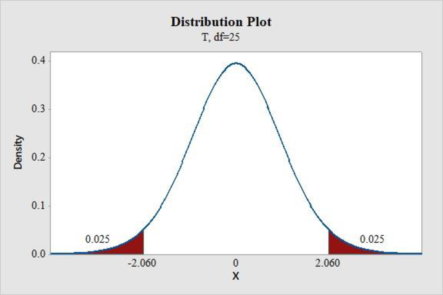
From the MINITAB output, the critical value is 2.060.
From the given MINITAB output, the value of
The confidence interval for mean change in exam score is calculated as follows:
Thus, the 95% confidence interval for
There is 95% confident that the average increase in y is associated with 1-unit increase in starch damage that is between 0.298 and 0.373, when the other predictors are fixed.
c.
- i. Test the hypothesis
H 0 : β 1 = 0 H a : β 1 ≠ 0
- ii. Test the hypothesis
H 0 : β 2 = 0 H a : β 2 ≠ 0
c.
Answer to Problem 46E
It can be concluded that the quadratic term should not be eliminated from the model and simple linear model should not be sufficient.
Explanation of Solution
Calculation:
i.
1.
The predictor
2.
Null hypothesis:
3.
Alternative hypothesis:
4.
Here, the common significance levels are
5.
Test statistic:
Here,
6.
Assumptions:
The random deviations from the values by the population regression equation are distributed normally with mean 0 and fixed standard deviation.
7.
Calculation:
From the MINITAB output, the t test statistic value of
8.
P-value:
From the MINITAB output, the P-value for
9.
Conclusion:
If the
Therefore, the P-value of 0 is less than any common levels of significance, such as 0.05, 0.01, and 0.10.
Hence, reject the null hypothesis.
Thus, there is convincing evidence that the flour protein variable is important and it is
ii.
1.
The predictor
2.
Null hypothesis:
3.
Alternative hypothesis:
4.
Here, the common significance levels are
5.
Test statistic:
Here,
6.
Assumptions:
The random deviations from the values by the population regression equation are distributed normally with mean 0 and fixed standard deviation.
7.
Calculation:
From the MINITAB output, the t test statistic value of
8.
P-value:
From the MINITAB output, the P-value for
9.
Conclusion:
If the
Therefore, the P-value of 0 is less than any common levels of significance, such as 0.05, 0.01, and 0.10.
Hence, reject the null hypothesis.
Thus, there is convincing evidence that the starch damage variable is important and it is
d.
Explain whether both the independent variables are important or not.
d.
Explanation of Solution
From the results of Part (c), there is evidence that the variables of flour protein and starch damage are important.
e.
Calculate a 90% confidence interval and interpret it.
e.
Answer to Problem 46E
The 90% confidence interval is
Explanation of Solution
Calculation:
It is given that the value of
Assume that the exam score is associated with the predictors according to the model. The random deviations from the values by the population regression equation are distributed normally with mean 0 and fixed standard deviation.
The formula for prediction interval for mean y value is as follows:
The value of
Degrees of freedom:
Software procedure:
Step-by-step procedure to find the P-value using the MINITAB software:
- Choose Graph > Probability Distribution Plot choose View Probability > OK.
- From Distribution, choose ‘t’ distribution.
- Enter the Degrees of freedom as 25.
- Click the Shaded Area tab.
- Choose Probability and Both for the region of the curve to shade.
- Enter the Probability value as 0.10.
- Click OK.
Output obtained using the MINITAB software is represented as follows:
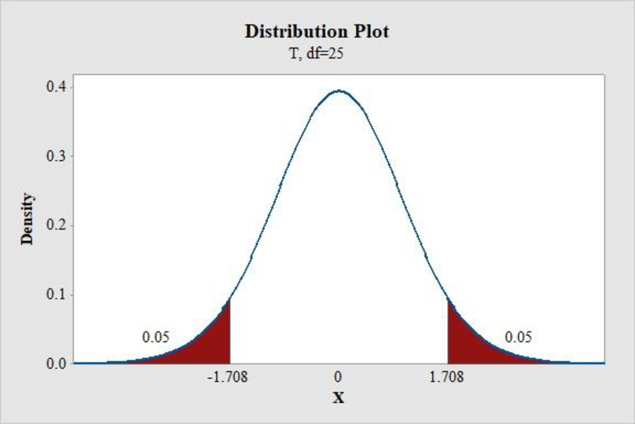
From the MINITAB output, the critical value is 1.708.
The prediction interval for mean y value is calculated as follows:
Thus, the 90% confidence interval is
There is 90% confident that the mean water absorption for wheat with 11.7 flour protein and 57 starch damage is between 54.5084 and 56.2916.
f.
Predict the water absorption for the shipment by 90% interval.
f.
Answer to Problem 46E
The water absorption values for the particular shipment are between 53.3297 and 57.4703 by 90% prediction interval.
Explanation of Solution
Calculation:
It is given that the value of
Assume that the exam score is associated with the predictors according to the model. The random deviations from the values by the population regression equation are distributed normally with mean 0 and fixed standard deviation.
The formula for prediction interval for mean y value is as follows:
From the given MINITAB output, the standard deviation is 1.094.
From Part e., the value of
From the MINITAB output in Part e., the critical value is 1.708.
The prediction interval for water absorption for shipment is calculated as follows:
Thus, the 90% prediction interval is
By prediction at 90% interval, the water absorption values for the particular shipment are between 53.3297 and 57.4703.
Want to see more full solutions like this?
Chapter 14 Solutions
Introduction to Statistics and Data Analysis


- Harvard University California Institute of Technology Massachusetts Institute of Technology Stanford University Princeton University University of Cambridge University of Oxford University of California, Berkeley Imperial College London Yale University University of California, Los Angeles University of Chicago Johns Hopkins University Cornell University ETH Zurich University of Michigan University of Toronto Columbia University University of Pennsylvania Carnegie Mellon University University of Hong Kong University College London University of Washington Duke University Northwestern University University of Tokyo Georgia Institute of Technology Pohang University of Science and Technology University of California, Santa Barbara University of British Columbia University of North Carolina at Chapel Hill University of California, San Diego University of Illinois at Urbana-Champaign National University of Singapore McGill…arrow_forwardName Harvard University California Institute of Technology Massachusetts Institute of Technology Stanford University Princeton University University of Cambridge University of Oxford University of California, Berkeley Imperial College London Yale University University of California, Los Angeles University of Chicago Johns Hopkins University Cornell University ETH Zurich University of Michigan University of Toronto Columbia University University of Pennsylvania Carnegie Mellon University University of Hong Kong University College London University of Washington Duke University Northwestern University University of Tokyo Georgia Institute of Technology Pohang University of Science and Technology University of California, Santa Barbara University of British Columbia University of North Carolina at Chapel Hill University of California, San Diego University of Illinois at Urbana-Champaign National University of Singapore…arrow_forwardA company found that the daily sales revenue of its flagship product follows a normal distribution with a mean of $4500 and a standard deviation of $450. The company defines a "high-sales day" that is, any day with sales exceeding $4800. please provide a step by step on how to get the answers in excel Q: What percentage of days can the company expect to have "high-sales days" or sales greater than $4800? Q: What is the sales revenue threshold for the bottom 10% of days? (please note that 10% refers to the probability/area under bell curve towards the lower tail of bell curve) Provide answers in the yellow cellsarrow_forward
- Find the critical value for a left-tailed test using the F distribution with a 0.025, degrees of freedom in the numerator=12, and degrees of freedom in the denominator = 50. A portion of the table of critical values of the F-distribution is provided. Click the icon to view the partial table of critical values of the F-distribution. What is the critical value? (Round to two decimal places as needed.)arrow_forwardA retail store manager claims that the average daily sales of the store are $1,500. You aim to test whether the actual average daily sales differ significantly from this claimed value. You can provide your answer by inserting a text box and the answer must include: Null hypothesis, Alternative hypothesis, Show answer (output table/summary table), and Conclusion based on the P value. Showing the calculation is a must. If calculation is missing,so please provide a step by step on the answers Numerical answers in the yellow cellsarrow_forwardShow all workarrow_forward
 MATLAB: An Introduction with ApplicationsStatisticsISBN:9781119256830Author:Amos GilatPublisher:John Wiley & Sons Inc
 Probability and Statistics for Engineering and th...StatisticsISBN:9781305251809Author:Jay L. DevorePublisher:Cengage Learning
 Statistics for The Behavioral Sciences (MindTap C...StatisticsISBN:9781305504912Author:Frederick J Gravetter, Larry B. WallnauPublisher:Cengage Learning
 Elementary Statistics: Picturing the World (7th E...StatisticsISBN:9780134683416Author:Ron Larson, Betsy FarberPublisher:PEARSON
 The Basic Practice of StatisticsStatisticsISBN:9781319042578Author:David S. Moore, William I. Notz, Michael A. FlignerPublisher:W. H. Freeman
 Introduction to the Practice of StatisticsStatisticsISBN:9781319013387Author:David S. Moore, George P. McCabe, Bruce A. CraigPublisher:W. H. Freeman