Match the data series from the options shown on the graph to the following model types. You may assume that power and exponential models do not have a constant offset. You may also assume that only positive values are shown on the two axes. For each match, write “Series X.” where X is the appropriate letter, A through F. If no curve matches the specified criterion, write “No Match.” If more than one curve matches a given specification, list both series.
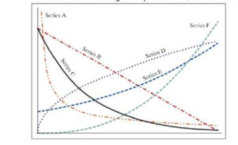
- a. Exponential, negative numeric value in exponent
- b. Power, negative numeric value in exponent
- c. Linear, negative slope
- d. Exponential, positive numeric value in exponent
- e. Power, positive numeric value in exponent
Want to see the full answer?
Check out a sample textbook solution
Chapter 12 Solutions
Thinking Like an Engineer: An Active Learning Approach (4th Edition)
Additional Engineering Textbook Solutions
Starting Out with Programming Logic and Design (5th Edition) (What's New in Computer Science)
Thermodynamics: An Engineering Approach
Problem Solving with C++ (10th Edition)
Vector Mechanics for Engineers: Statics and Dynamics
Fluid Mechanics: Fundamentals and Applications
Database Concepts (8th Edition)
- During some actual expansion and compression processes in piston–cylinder devices, the gases have been observed to satisfy the relationship PVn = C, where n and C are constants. Calculate the work done when a gas expands from 350 kPa and 0.03 m3 to a final volume of 0.2 m3 for the case of n = 1.5. The work done in this case is kJ.arrow_forwardCarbon dioxide contained in a piston–cylinder device is compressed from 0.3 to 0.1 m3. During the process, the pressure and volume are related by P = aV–2, where a = 6 kPa·m6. Calculate the work done on carbon dioxide during this process. The work done on carbon dioxide during this process is kJ.arrow_forwardThe volume of 1 kg of helium in a piston–cylinder device is initially 5 m3. Now helium is compressed to 3 m3 while its pressure is maintained constant at 130 kPa. Determine the initial and final temperatures of helium as well as the work required to compress it, in kJ. The gas constant of helium is R = 2.0769 kJ/kg·K. The initial temperature of helium is K. The final temperature of helium is K. The work required to compress helium is kJ.arrow_forward
- A piston-cylinder device initially contains 0.4 kg of nitrogen gas at 160 kPa and 140°C. Nitrogen is now expanded isothermally to a pressure of 80 kPa. Determine the boundary work done during this process. The properties of nitrogen are R= 0.2968 kJ/kg-K and k= 1.4. N₂ 160 kPa 140°C The boundary work done during this process is KJ.arrow_forward! Required information An abrasive cutoff wheel has a diameter of 5 in, is 1/16 in thick, and has a 3/4-in bore. The wheel weighs 4.80 oz and runs at 11,700 rev/min. The wheel material is isotropic, with a Poisson's ratio of 0.20, and has an ultimate strength of 12 kpsi. Choose the correct equation from the following options: Multiple Choice о σmax= (314) (4r2 — r²) - о σmax = p² (3+) (4r² + r²) 16 σmax = (314) (4r² + r²) σmax = (314) (4² - r²)arrow_forwardI don't know how to solve thisarrow_forward
- I am not able to solve this question. Each part doesn't make sense to me.arrow_forwardExercises Find the solution of the following Differential Equations 1) y" + y = 3x² 3) "+2y+3y=27x 5) y"+y=6sin(x) 7) y"+4y+4y = 18 cosh(x) 9) (4)-5y"+4y = 10 cos(x) 11) y"+y=x²+x 13) y"-2y+y=e* 15) y+2y"-y'-2y=1-4x³ 2) y"+2y' + y = x² 4) "+y=-30 sin(4x) 6) y"+4y+3y=sin(x)+2 cos(x) 8) y"-2y+2y= 2e* cos(x) 10) y+y-2y=3e* 12) y"-y=e* 14) y"+y+y=x+4x³ +12x² 16) y"-2y+2y=2e* cos(x)arrow_forwardQu. 15 What are the indices for the Plane 1 drawn in the following sketch? Qu. 16 What are the Miller indices for the Plane shown in the following cubic unit cell? this is material engineering please show all workarrow_forward
 Elements Of ElectromagneticsMechanical EngineeringISBN:9780190698614Author:Sadiku, Matthew N. O.Publisher:Oxford University Press
 Mechanics of Materials (10th Edition)Mechanical EngineeringISBN:9780134319650Author:Russell C. HibbelerPublisher:PEARSON
 Thermodynamics: An Engineering ApproachMechanical EngineeringISBN:9781259822674Author:Yunus A. Cengel Dr., Michael A. BolesPublisher:McGraw-Hill Education
 Control Systems EngineeringMechanical EngineeringISBN:9781118170519Author:Norman S. NisePublisher:WILEY
 Mechanics of Materials (MindTap Course List)Mechanical EngineeringISBN:9781337093347Author:Barry J. Goodno, James M. GerePublisher:Cengage Learning
 Engineering Mechanics: StaticsMechanical EngineeringISBN:9781118807330Author:James L. Meriam, L. G. Kraige, J. N. BoltonPublisher:WILEY

