
Concept explainers
Videos
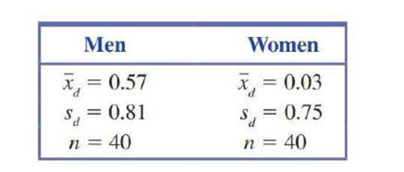
The paper “The Truth About Lying in Online Dating Profiles” (Proceedings, Computer-Human Interaction [2007]: 1–4) describes an investigation in which 40 men and 40 women with online dating profiles agreed to participate in a study. Each participant’s height (in inches) was measured and the actual height was compared to the height given in that person’s online profile. The differences between the online profile height and the actual height (profile – actual) were used to calculate the values in the accompanying table.
You can assume it is reasonable to regard the two samples in this study as being representative of male online daters and female online daters. (Although the authors of the paper believed that their samples were representative of these populations, participants were volunteers recruited through newspaper advertisements, so we should be a bit hesitant to generalize results to all online daters.)
- a. Use the paired t test to determine if there is convincing evidence that, on average, male online daters overstate their height in online dating profiles. Use α = 0.05.
- b. Construct and interpret a 95% confidence interval for the difference between the
mean online dating profile height and mean actual height for female online daters. (Hint: See Example 11.8.) - c. Use the two-sample t test of Section 11.1 to test H0: μm – μf = 0 versus Ha: μm – μf > 0, where μm is the mean height difference (profile – actual) for male online daters and μf, is the mean height difference (profile – actual) for female online daters.
- d. Explain why a paired t test was used in Part (a) but a two-sample t test was used in Part (c).
a.
Check whether there is convincing evidence that the average male online daters overstate their height in online dating profile or not.
Answer to Problem 29E
There is convincing evidence that the average male online daters overstate their height in online dating profile.
Explanation of Solution
Calculation:
Total of 40 men and 40 women are sampled. The sample size, standard deviation, and mean for diference between profile height and actual height, for men and women are given.
Assumption for conducting the test:
- The sample difference should be a random sample.
- The population distribution for the mean differences should follow approximately normal distribution.
- The samples are paired.
Here, the samples are paired. It is reasonable to assume that the two samples of men and women acts as the representative for all the male online daters and female online daters.
Let
Let
Here,
That is,
Hypotheses:
Null hypothesis:
That is, the mean difference between profile height and actual height, for men is zero.
Alternative hypothesis:
That is, the mean difference between profile height and actual height is greater than zero.
Test statistic:
Software procedure:
Step by step procedure to obtain the test statistic by using MINITAB software is given below:
- Choose Stat > Basic Statistics > Paired t.
- Choose summarized data.
- In choose sample size as 40, means as 0.57 and standard deviation as 0.81.
- Choose Options.
- In Confidence level, enter 95.
- In Alternative, select greater than.
- Click OK in all dialogue boxes.
Output using the MINITAB software is given below:
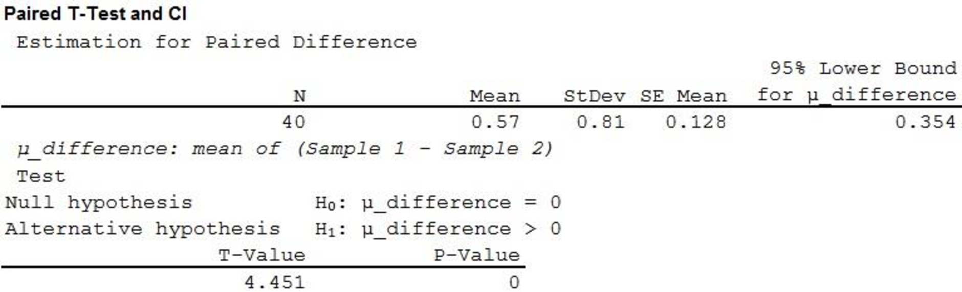
From the above MINITAB output the test statistic is 4.451 and the P-value is 0.
Decision rule:
- If P-value is less than or equal to the level of significance, reject the null hypothesis.
- Otherwise fail to reject the null hypothesis.
Conclusion:
Here, the level of significance is 0.05.
Here, P-value is less than the level of significance.
That is,
Therefore, reject the null hypothesis.
It can be concluded that there is convincing evidence that the average male online daters overstate their height in online dating profile.
b.
Construct a 95% confidence interval for the difference in mean profile height and mean actual height for female online daters.
Interpret the interval.
Answer to Problem 29E
The 95% confidence interval for the difference in mean profile height and mean actual height for female online daters is
Explanation of Solution
Calculation:
Assumptions for conducting the hypothesis test:
- The sample difference should be a random sample.
- The population distribution for the mean differences should follow approximately normal distribution.
- The samples are paired.
Here, samples are paired. The selected samples were representatives of population. Since the sample size is large
Confidence interval:
Software procedure:
Step by step procedure to obtain the confidence interval by using MINITAB software is as follows:
- Choose Stat > Basic Statistics > Paired t.
- Choose summarized data.
- In choose sample size as 40, means as 0.03 and standard deviation as 0.75.
- Choose Options.
- In Confidence level, enter 95.
- In Alternative, select not equal.
- Click OK in all dialogue boxes.
Output using the MINITAB software is given below:
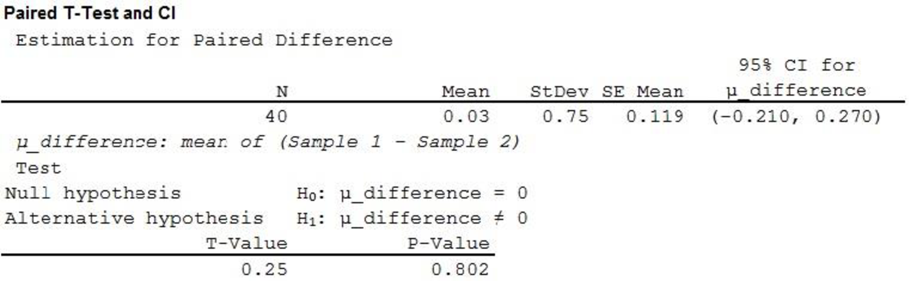
From the output, the 95% confidence interval is
Interpretation:
One can be 95% confident that the difference in mean profile height and mean actual height for female online daters lies between –0.210 and 0.270.
c.
Conduct a two sample t-test.
Answer to Problem 29E
There is convincing evidence that the mean height difference is higher for males than females.
Explanation of Solution
Calculation:
In this context, two sample t-test is used for the comparison.
Assumption for the two sample t-test:
- The random samples should be collected independently.
- The sample sizes should be large. That is, each sample size is at least 30. Or the populations are approximately normally distributed.
Requirement check:
Here, samples are selected at random from the population. Each sample has size of 40, which is greater than 30.
Therefore, the assumptions are satisfied.
Let
Let
Hypotheses:
Null hypothesis:
That is, the mean height difference is same for both males and females.
Alternative hypothesis:
That is, the mean height difference is higher for males than females.
Test statistic and P-value:
Software procedure:
Step by step procedure to obtain the P-value and test statistic by using MINITAB software:
- Choose Stat > Basic Statistics > 2 sample t.
- Choose Summarized data.
- In sample 1, enter Sample size as 40, Mean as 0.57, Standard deviation as 0.03.
- In sample 2, enter Sample size as 40, Mean as 0.03, Standard deviation as 0.75.
- Choose Options.
- In Confidence level, enter 95.
- In Alternative, select greater than.
- Click OK in all the dialogue boxes.
Output using the MINITAB software is given below:
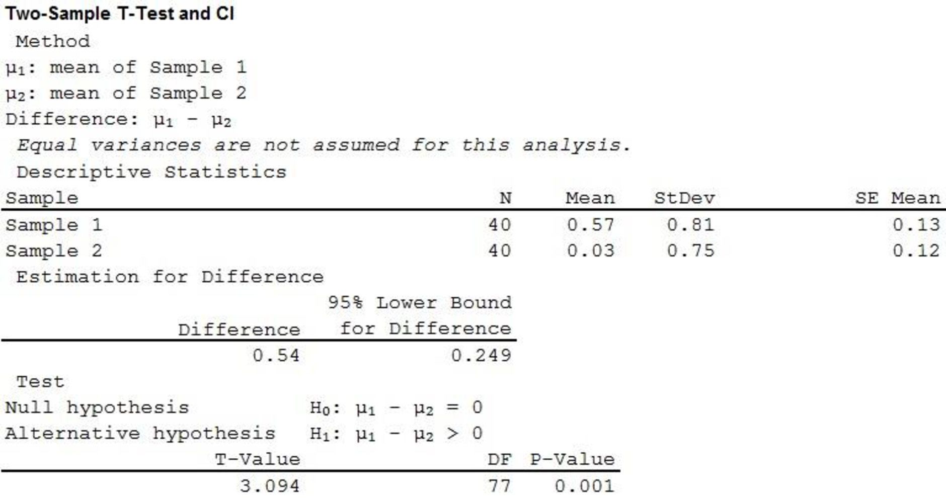
Therefore, the P-value is 0.001 and the test statistic is 3.094.
Decision rule:
- If P-value is less than or equal to the level of significance, reject the null hypothesis.
- Otherwise fail to reject the null hypothesis.
Conclusion:
Here, the level of significance is 0.05.
Here, P-value is less than the level of significance.
That is,
Therefore, reject the null hypothesis.
Hence, it can be concluded that there is convincing evidence that the mean height difference is higher for males than females.
d.
Explain the reason for paired t test was used in Part (a) two sample t-test was used in Part (c).
Explanation of Solution
Calculation:
In this context, the result obtained in Part (a) compares the mean actual and profile height for males. That is, the male profile and actual heights are paired. Therefore, the paired t test was used in Part (a).
Now, in this case, the result obtained in Part (c) compares the mean height difference for male and female. That is, the samples of male and female are independent. Therefore, the two sample t-test was used in Part (c).
Want to see more full solutions like this?
Chapter 11 Solutions
Introduction to Statistics and Data Analysis


- Suppose a random sample of 459 married couples found that 307 had two or more personality preferences in common. In another random sample of 471 married couples, it was found that only 31 had no preferences in common. Let p1 be the population proportion of all married couples who have two or more personality preferences in common. Let p2 be the population proportion of all married couples who have no personality preferences in common. Find a95% confidence interval for . Round your answer to three decimal places.arrow_forwardA history teacher interviewed a random sample of 80 students about their preferences in learning activities outside of school and whether they are considering watching a historical movie at the cinema. 69 answered that they would like to go to the cinema. Let p represent the proportion of students who want to watch a historical movie. Determine the maximal margin of error. Use α = 0.05. Round your answer to three decimal places. arrow_forwardA random sample of medical files is used to estimate the proportion p of all people who have blood type B. If you have no preliminary estimate for p, how many medical files should you include in a random sample in order to be 99% sure that the point estimate will be within a distance of 0.07 from p? Round your answer to the next higher whole number.arrow_forward
- A clinical study is designed to assess the average length of hospital stay of patients who underwent surgery. A preliminary study of a random sample of 70 surgery patients’ records showed that the standard deviation of the lengths of stay of all surgery patients is 7.5 days. How large should a sample to estimate the desired mean to within 1 day at 95% confidence? Round your answer to the whole number.arrow_forwardA clinical study is designed to assess the average length of hospital stay of patients who underwent surgery. A preliminary study of a random sample of 70 surgery patients’ records showed that the standard deviation of the lengths of stay of all surgery patients is 7.5 days. How large should a sample to estimate the desired mean to within 1 day at 95% confidence? Round your answer to the whole number.arrow_forwardIn the experiment a sample of subjects is drawn of people who have an elbow surgery. Each of the people included in the sample was interviewed about their health status and measurements were taken before and after surgery. Are the measurements before and after the operation independent or dependent samples?arrow_forward
- iid 1. The CLT provides an approximate sampling distribution for the arithmetic average Ỹ of a random sample Y₁, . . ., Yn f(y). The parameters of the approximate sampling distribution depend on the mean and variance of the underlying random variables (i.e., the population mean and variance). The approximation can be written to emphasize this, using the expec- tation and variance of one of the random variables in the sample instead of the parameters μ, 02: YNEY, · (1 (EY,, varyi n For the following population distributions f, write the approximate distribution of the sample mean. (a) Exponential with rate ẞ: f(y) = ß exp{−ßy} 1 (b) Chi-square with degrees of freedom: f(y) = ( 4 ) 2 y = exp { — ½/ } г( (c) Poisson with rate λ: P(Y = y) = exp(-\} > y! y²arrow_forward2. Let Y₁,……., Y be a random sample with common mean μ and common variance σ². Use the CLT to write an expression approximating the CDF P(Ỹ ≤ x) in terms of µ, σ² and n, and the standard normal CDF Fz(·).arrow_forwardmatharrow_forward
- Compute the median of the following data. 32, 41, 36, 42, 29, 30, 40, 22, 25, 37arrow_forwardTask Description: Read the following case study and answer the questions that follow. Ella is a 9-year-old third-grade student in an inclusive classroom. She has been diagnosed with Emotional and Behavioural Disorder (EBD). She has been struggling academically and socially due to challenges related to self-regulation, impulsivity, and emotional outbursts. Ella's behaviour includes frequent tantrums, defiance toward authority figures, and difficulty forming positive relationships with peers. Despite her challenges, Ella shows an interest in art and creative activities and demonstrates strong verbal skills when calm. Describe 2 strategies that could be implemented that could help Ella regulate her emotions in class (4 marks) Explain 2 strategies that could improve Ella’s social skills (4 marks) Identify 2 accommodations that could be implemented to support Ella academic progress and provide a rationale for your recommendation.(6 marks) Provide a detailed explanation of 2 ways…arrow_forwardQuestion 2: When John started his first job, his first end-of-year salary was $82,500. In the following years, he received salary raises as shown in the following table. Fill the Table: Fill the following table showing his end-of-year salary for each year. I have already provided the end-of-year salaries for the first three years. Calculate the end-of-year salaries for the remaining years using Excel. (If you Excel answer for the top 3 cells is not the same as the one in the following table, your formula / approach is incorrect) (2 points) Geometric Mean of Salary Raises: Calculate the geometric mean of the salary raises using the percentage figures provided in the second column named “% Raise”. (The geometric mean for this calculation should be nearly identical to the arithmetic mean. If your answer deviates significantly from the mean, it's likely incorrect. 2 points) Starting salary % Raise Raise Salary after raise 75000 10% 7500 82500 82500 4% 3300…arrow_forward
 Glencoe Algebra 1, Student Edition, 9780079039897...AlgebraISBN:9780079039897Author:CarterPublisher:McGraw Hill
 Big Ideas Math A Bridge To Success Algebra 1: Stu...AlgebraISBN:9781680331141Author:HOUGHTON MIFFLIN HARCOURTPublisher:Houghton Mifflin Harcourt
 College Algebra (MindTap Course List)AlgebraISBN:9781305652231Author:R. David Gustafson, Jeff HughesPublisher:Cengage Learning
 Holt Mcdougal Larson Pre-algebra: Student Edition...AlgebraISBN:9780547587776Author:HOLT MCDOUGALPublisher:HOLT MCDOUGAL