Chapter 11, Problem 61CR

a.

To determine

Check whether there is sufficient evidence to conclude that the mean “appropriateness” score assigned to wearing a hat in class differs for students and faculty.

Answer to Problem 61CR

The conclusion is that there is sufficient evidence to conclude that the mean “appropriateness” score assigned to wearing a hat in class differs for students and faculty.

Explanation of Solution

Calculation:

$n_1=173$, $n_2=98$, ${\overline{x}}_1=2.80$, ${\overline{x}}_2=3.63$, $s_1=1.0$, and $s_2=1.0$.

Step 1:

In this context, ${\mu }_1$ denotes the mean “appropriateness” score assigned to wearing a hat in class for students and ${\mu }_2$ denotes the mean “appropriateness” score assigned to wearing a hat in class for faculty.

Step 2:

Null hypothesis:

$H_0:{\mu }_1-{\mu }_2=0$

Step 3:

Alternative hypothesis:

$H_a:{\mu }_1-{\mu }_2\ne 0$

Step 4:

Significance level, $\alpha$:

It is given that the significance level, $\alpha =0.05$.

Step 5:

Test statistic:

$\begin{array}{c}t=\frac{\left({\overline{x}}_1-{\overline{x}}_2\right)-\text{hypothesized value}}{\sqrt{\frac{s_1^2}{n_1}+\frac{s_2^2}{n_2}}}\\ =\frac{\left({\overline{x}}_1-{\overline{x}}_2\right)-0}{\sqrt{\frac{s_1^2}{n_1}+\frac{s_2^2}{n_2}}}\end{array}$

Step 6:

The assumption for the two-sample t-test:

• The random samples should be collected independently.
• The sample sizes should be large. That is, each sample size is at least 30.

The assumptions in this particular problem are as follows:

• Data are collected independently.
• The sample sizes are large. That is, both sample sizes are greater than 30.

Therefore, the assumptions are satisfied.

Step 7:

Test statistic:

Software procedure:

Step-by-step procedure to obtain the P-value and test statistic by using MINITAB software:

• Choose Stat > Basic Statistics > 2 sample t.
• Choose Summarized data.
• In sample 1, enter Sample size as 173, Mean as 2.80, Standard deviation as 1.
• In sample 2, enter Sample size as 98, Mean as 3.63, Standard deviation as 1.
• Choose Options.
• In Confidence level, enter 95.
• In Alternative, select not equal.
• Click OK in all the dialogue boxes.

Output obtained using the MINITAB software is given below:

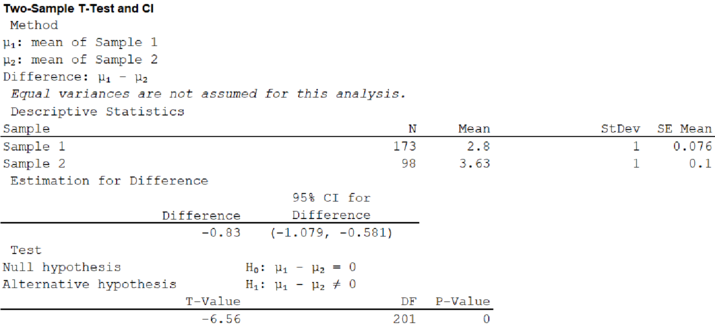
From the given MINITAB output, the value of test statistic is –6.56.

Step 8:

P-value:

From the MINITAB output, the P-value is 0.

Step 9:

Decision rule:

If $P\text{-value}\le \alpha$, then reject the null hypothesis $H_0$.

Conclusion:

Here, the $P\text{-value}$ of 0 is less than the significance level 0.05.

That is, $P\text{-value}\left(=0\right)<\alpha \left(=0.05\right)$.

The decision is that the null hypothesis is rejected.

Hence, there is sufficient evidence to conclude that the mean “appropriateness” score assigned to wearing a hat in class differs for students and faculty.

b.

To determine

Check whether there is sufficient evidence to conclude that the mean “appropriateness” score assigned to addressing an instructor by his or her first name is greater for students than for faculty.

Answer to Problem 61CR

The conclusion is that there is sufficient evidence to conclude that the mean “appropriateness” score assigned to addressing an instructor by his or her first name is greater for students than for faculty.

Explanation of Solution

Calculation:

$n_1=173$, $n_2=98$, ${\overline{x}}_1=2.90$, ${\overline{x}}_2=2.11$, $s_1=1.0$, and $s_2=1.0$.

Step 1:

In this context, ${\mu }_1$ denotes the mean “appropriateness” score assigned to addressing an instructor by his or her first name for students and ${\mu }_2$ denotes the mean “appropriateness” score assigned to addressing an instructor by his or her first name for faculty.

Step 2:

Null hypothesis:

$H_0:{\mu }_1-{\mu }_2=0$

Step 3:

Alternative hypothesis:

$H_a:{\mu }_1-{\mu }_2>0$

Step 4:

Significance level, $\alpha$:

It is given that the significance level, $\alpha =0.05$.

Step 5:

Test statistic:

$\begin{array}{c}t=\frac{\left({\overline{x}}_1-{\overline{x}}_2\right)-\text{hypothesized value}}{\sqrt{\frac{s_1^2}{n_1}+\frac{s_2^2}{n_2}}}\\ =\frac{\left({\overline{x}}_1-{\overline{x}}_2\right)-0}{\sqrt{\frac{s_1^2}{n_1}+\frac{s_2^2}{n_2}}}\end{array}$

Step 6:

The assumption for the two-sample t-test:

• The random samples should be collected independently.
• The sample sizes should be large. That is, each sample size is at least 30.

The assumptions in this particular problem are as follows:

• Data are collected independently.
• The sample sizes are large. That is, both sample sizes are greater than 30.

Therefore, the assumptions are satisfied.

Step 7:

Test statistic:

Software procedure:

Step-by-step procedure to obtain the P-value and test statistic by using MINITAB software:

• Choose Stat > Basic Statistics > 2 sample t.
• Choose Summarized data.
• In sample 1, enter Sample size as 173, Mean as 2.90, Standard deviation as 1.
• In sample 2, enter Sample size as 98, Mean as 2.11, Standard deviation as 1.
• Choose Options.
• In Confidence level, enter 95.
• In Alternative, select greater than.
• Click OK in all the dialogue boxes.

Output obtained using the MINITAB software is given below:

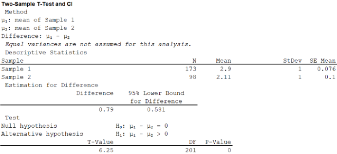
From the given MINITAB output, the value of test statistic is 6.25.

Step 8:

P-value:

From the MINITAB output, the P-value is 0.

Step 9:

Decision rule:

If $P\text{-value}\le \alpha$, then reject the null hypothesis $H_0$.

Conclusion:

Here, the $P\text{-value}$ of 0 is less than the significance level 0.05.

That is, $P\text{-value}\left(=0\right)<\alpha \left(=0.05\right)$.

The decision is that the null hypothesis is rejected.

Hence, there is sufficient evidence to conclude that the mean “appropriateness” score assigned to addressing an instructor by his or her first name is greater for students than for faculty.

c.

To determine

Check whether there is sufficient evidence to conclude that the mean “appropriateness” score assigned to talking on a cell phone differs for students and faculty.

Answer to Problem 61CR

The conclusion is that there is no sufficient evidence to conclude that the mean “appropriateness” score assigned to talking on a cell phone differs for students and faculty.

Explanation of Solution

Calculation:

$n_1=173$, $n_2=98$, ${\overline{x}}_1=1.11$, ${\overline{x}}_2=1.10$, $s_1=1.0$, and $s_2=1.0$.

Step 1:

In this context, ${\mu }_1$ denotes the mean “appropriateness” score assigned to talking on a cell phone for students and ${\mu }_2$ denotes the mean “appropriateness” score assigned to talking on a cell phone for faculty.

Step 2:

Null hypothesis:

$H_0:{\mu }_1-{\mu }_2=0$

Step 3:

Alternative hypothesis:

$H_a:{\mu }_1-{\mu }_2\ne 0$

Step 4:

Significance level, $\alpha$:

It is given that the significance level, $\alpha =0.05$.

Step 5:

Test statistic:

$\begin{array}{c}t=\frac{\left({\overline{x}}_1-{\overline{x}}_2\right)-\text{hypothesized value}}{\sqrt{\frac{s_1^2}{n_1}+\frac{s_2^2}{n_2}}}\\ =\frac{\left({\overline{x}}_1-{\overline{x}}_2\right)-0}{\sqrt{\frac{s_1^2}{n_1}+\frac{s_2^2}{n_2}}}\end{array}$

Step 6:

The assumption for the two-sample t-test:

• The random samples should be collected independently.
• The sample sizes should be large. That is, each sample size is at least 30.

The assumptions in this particular problem are as follows:

• Data are collected independently.
• The sample sizes are large. That is, both sample sizes are greater than 30.

Therefore, the assumptions are satisfied.

Step 7:

Test statistic:

Software procedure:

Step-by-step procedure to obtain the P-value and test statistic by using MINITAB software:

• Choose Stat > Basic Statistics > 2 sample t.
• Choose Summarized data.
• In sample 1, enter Sample size as 173, Mean as 1.11, Standard deviation as 1.
• In sample 2, enter Sample size as 98, Mean as 1.10, Standard deviation as 1.
• Choose Options.
• In Confidence level, enter 95.
• In Alternative, select not equal.
• Click OK in all the dialogue boxes.

Output obtained using the MINITAB software is given below:

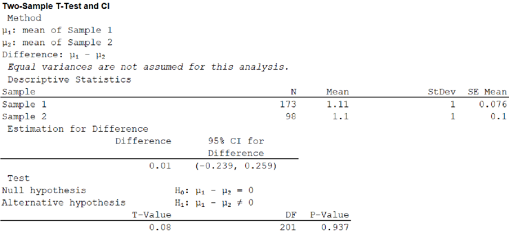
From the given MINITAB output, the value of test statistic is 0.08.

Step 8:

P-value:

From the MINITAB output, the P-value is 0.937.

Step 9:

Decision rule:

If $P\text{-value}\le \alpha$, then reject the null hypothesis $H_0$.

Conclusion:

Here, the $P\text{-value}$ of 0.937 is greater than the significance level 0.05.

That is, $P\text{-value}\left(=0.937\right)>\alpha \left(=0.05\right)$.

The decision is that the null hypothesis is not rejected.

Hence, there is no sufficient evidence to conclude that the mean “appropriateness” score assigned to talking on a cell phone differs for students and faculty.

d.

To determine

Check whether the result of the test in part (c) imply that students and faculty consider that it is acceptable to talk on a cell phone during class.

Answer to Problem 61CR

No, the result of the test in part (c) does not imply that students and faculty consider that it is acceptable to talk on a cell phone during class.

Explanation of Solution

Here, the sample mean rating is lesser in both students and faculty. This shows that the behavior for the both groups is inappropriate. Hence, the result of the test in part (c) does not imply that students and faculty consider that it is acceptable to talk on a cell phone during class.