
Videos
a.
Check whether the data provide convincing support for the claim that, on average, male teenager drivers exceed the speed limit by more than do female teenage drivers.
a.
Answer to Problem 18E
The conclusion is that the data provide convincing support for the claim that, on average, male teenager drivers exceed the speed limit by more than do female teenage drivers.
Explanation of Solution
Calculation:
The data are based on the speed limit for male and female drivers.
Step 1:
In this context,
Step 2:
Null hypothesis:
Step 3:
Alternative hypothesis:
Step 4:
Significance level,
It is given that the significance level,
Step 5:
Test statistic:
Step 6:
The assumption for the two-sample t-test:
- The random samples should be collected independently.
- The sample sizes should be large. That is, each sample size is at least 30 or the populations are approximately normally distributed.
It is assumed that the distribution of the speed limit for male and female drivers is normally distributed.
Boxplot:
Software procedure:
Step-by-step procedure to obtain a boxplot using MINITAB software:
- Choose Graphs > Boxplot.
- Under Multiple Y’s, choose Simple.
- In Graph variables, enter the column of Male Driver and Female Driver.
- In Scale, choose Transpose values and categorical scales.
- Click OK in all dialogue boxes.
Output using MINITAB software is given below:
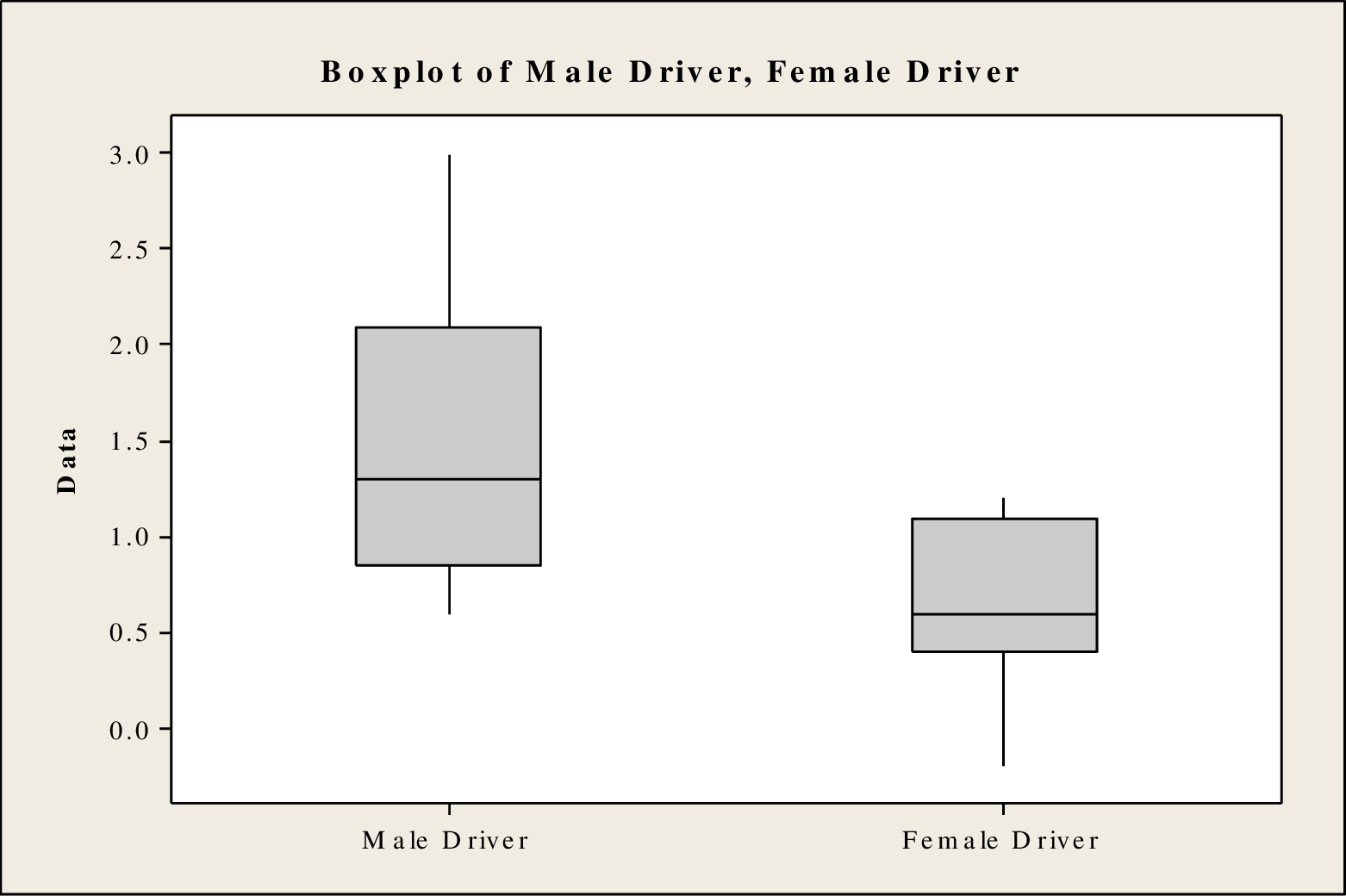
Any lack of symmetric that appears in the boxplot is acceptable for the given sample size because the sample size is larger.
From the boxplot, it is clear that the distribution of the speed limit for male drivers is skewed right and the distribution of the speed limit for female drivers is skewed left. Based on the sample size, the normality condition is satisfied. Morevoer, random samples are collected independently. Therefore, the assumptions are satisfied. It is reasonable to use the data for a two-sample t test.
Step 7:
Test statistic:
Software procedure:
Step-by-step procedure to obtain the P-value and test statistic using MINITAB software:
- Choose Stat > Basic Statistics > 2 sample t.
- Choose Samples in different columns.
- In sample 1, enter the column of Male Driver.
- In sample 2, enter the column of Female Driver.
- Choose Options.
- In Confidence level, enter 95.
- In Alternative, select greater than.
- Click OK in all the dialogue boxes.
Output obtained using MINITAB software is given below:
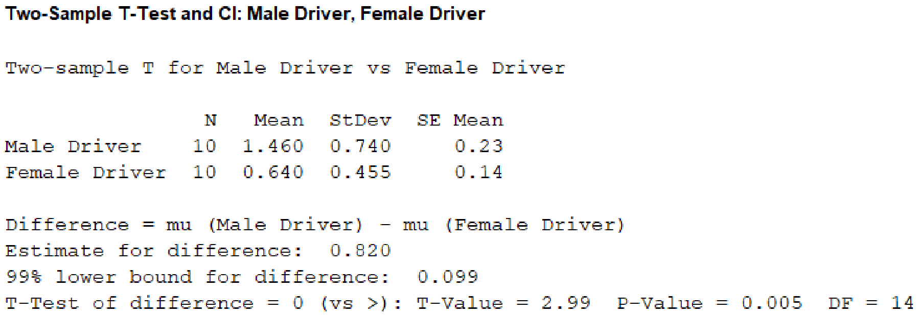
From the given MINITAB output, the value of the test statistic is 2.99.
Step 8:
P-value:
From the MINITAB output, the P-value is 0.005.
Step 9:
Decision rule:
If the
Here, the
That is,
The decision is that the null hypothesis is rejected.
Conclusion:
Hence, the data provide convincing support for the claim that, on average, male teenager drivers exceed the speed limit by more than do female teenage drivers.
b.
(i)
Check whether there is sufficient evidence to conclude that the average number of miles per hour over the speed limit is greater for male drivers with male passengers than it is for male drivers with female passengers.
(ii)
Check whether there is sufficient evidence to conclude that the average number of miles per hour over the speed limit is greater for female drivers with male passengers than it is for female drivers with female passengers.
(iii)
Check whether there is sufficient evidence to conclude that the average number of miles per hour over the speed limit is smaller for male drivers with female passengers than it is for female drivers with male passengers.
b.
Answer to Problem 18E
(i)
The conclusion is that there is sufficient evidence to conclude that the average number of miles per hour over the speed limit is greater for male drivers with male passengers than it is for male drivers with female passengers.
(ii)
The conclusion is that there is sufficient evidence to conclude that the average number of miles per hour over the speed limit is greater for female drivers with male passengers than it is for female drivers with female passengers.
(iii)
The conclusion is that there is sufficient evidence to conclude that the average number of miles per hour over the speed limit is smaller for male drivers with female passengers than it is for female drivers with male passengers.
Explanation of Solution
Calculation:
(i)
Step 1:
In this context,
Step 2:
Null hypothesis:
Step 3:
Alternative hypothesis:
Step 4:
Significance level,
It is given that the significance level
Step 5:
Test statistic:
Step 6:
Assumptions for the two-sample t-test:
- The random samples should be collected independently.
- The sample sizes should be large. That is, each sample size must be at least 30.
Assumption in this particular problem:
- Data are collected independently.
- The sample sizes are large.
Here, both sample sizes are greater than 30.
Therefore, the assumptions are satisfied.
Step 7:
Test statistic:
Software procedure:
Step-by-step procedure to obtain the P-value and test statistic using MINITAB software:
- Choose Stat > Basic Statistics > 2 sample t.
- Choose Summarized data.
- In sample 1, enter Sample size as 40, Mean as 5.2, Standard deviation as 0.8.
- In sample 2, enter Sample size as 40, Mean as 0.3, Standard deviation as 0.8.
- Choose Options.
- In Confidence level, enter 99.
- In Alternative, select greater than.
- Click OK in all the dialogue boxes.
Output obtained using MINITAB software is given below:
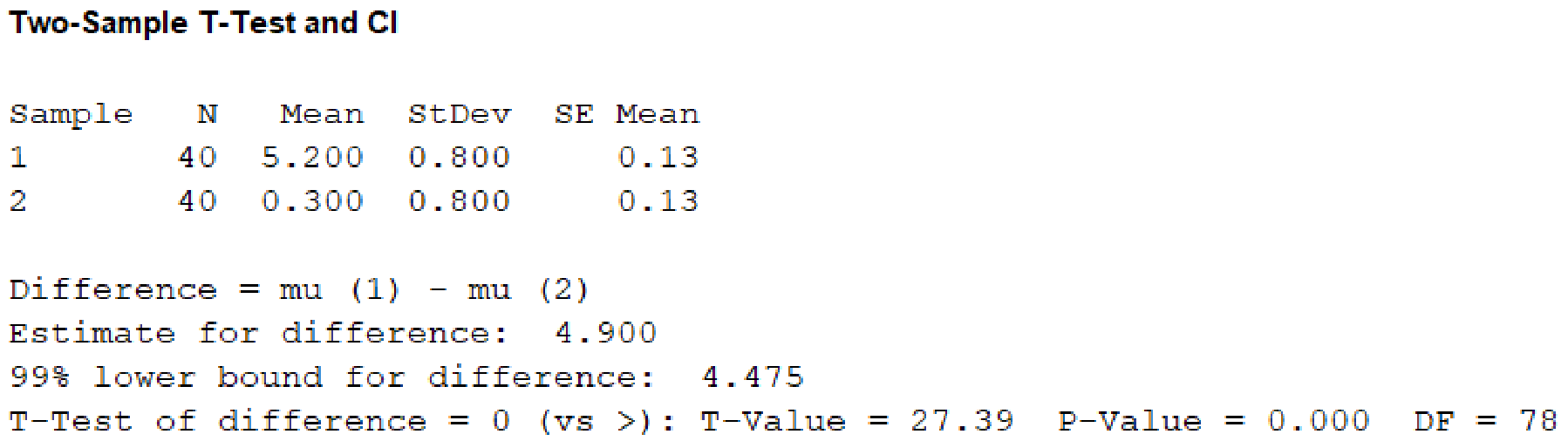
From the given MINITAB output, the value of test statistic is 27.39.
Step 8:
P-value:
From the MINITAB output, the P-value is 0.
Step 9:
Decision rule:
If the
Here, the
That is,
The decision is that the null hypothesis is rejected.
Conclusion:
Hence, there is sufficient evidence to conclude that the average number of miles per hour over the speed limit is greater for male drivers with male passengers than it is for male drivers with female passengers.
(ii)
Step 1:
In this context,
Step 2:
Null hypothesis:
Step 3:
Alternative hypothesis:
Step 4:
Significance level,
It is given that the significance level
Step 5:
Test statistic:
Step 6:
Assumptions for the two-sample t-test:
- The random samples should be collected independently.
- The sample sizes should be large. That is, each sample size must be at least 30.
Assumption in this particular problem:
- Data are collected independently.
- The sample sizes are large.
Here, both sample sizes are greater than 30.
Therefore, the assumptions are satisfied.
Step 7:
Test statistic:
Software procedure:
Step-by-step procedure to obtain the P-value and test statistic using MINITAB software:
- Choose Stat > Basic Statistics > 2 sample t.
- Choose Summarized data.
- In sample 1, enter Sample size as 40, Mean as 2.3, Standard deviation as 0.8.
- In sample 2, enter Sample size as 40, Mean as 0.6, Standard deviation as 0.8.
- Choose Options.
- In Confidence level, enter 99.
- In Alternative, select greater than.
- Click OK in all the dialogue boxes.
Output obtained using MINITAB software is given below:
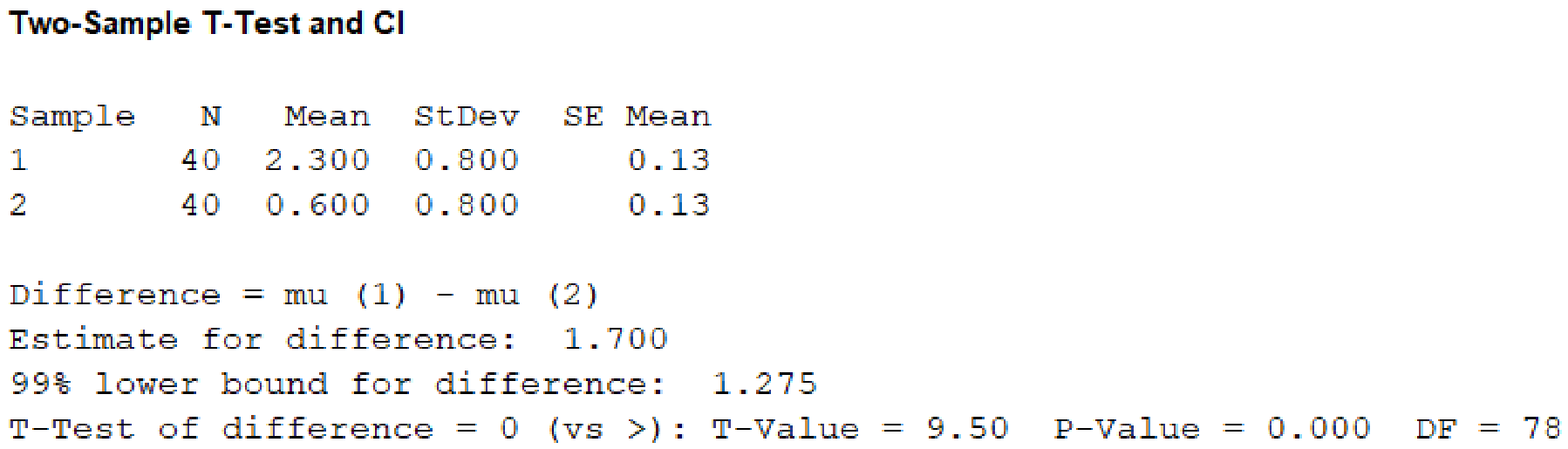
From the given MINITAB output, the value of test statistic is 9.50.
Step 8:
P-value:
From the MINITAB output, the P-value is 0.
Step 9:
Decision rule:
If the
Here, the
That is,
The decision is that the null hypothesis is rejected.
Conclusion:
Hence, there is sufficient evidence to conclude that the average number of miles per hour over the speed limit is greater for female drivers with male passengers than it is for female drivers with female passengers.
(iii)
Step 1:
In this context,
Step 2:
Null hypothesis:
Step 3:
Alternative hypothesis:
Step 4:
Significance level,
It is given that the significance level
Step 5:
Test statistic:
Step 6:
Assumptions for the two-sample t-test:
- The random samples should be collected independently.
- The sample sizes should be large. That is, each sample size must be at least 30.
Assumption in this particular problem:
- Data are collected independently.
- The sample sizes are large.
Here, both sample sizes are greater than 30.
Therefore, the assumptions are satisfied.
Step 7:
Test statistic:
Software procedure:
Step-by-step procedure to obtain the P-value and test statistic using MINITAB software:
- Choose Stat > Basic Statistics > 2 sample t.
- Choose Summarized data.
- In sample 1, enter Sample size as 40, Mean as 0.3, Standard deviation as 0.8.
- In sample 2, enter Sample size as 40, Mean as 2.3, Standard deviation as 0.8.
- Choose Options.
- In Confidence level, enter 99.
- In Alternative, select less than.
- Click OK in all the dialogue boxes.
Output obtained using the MINITAB software is given below:
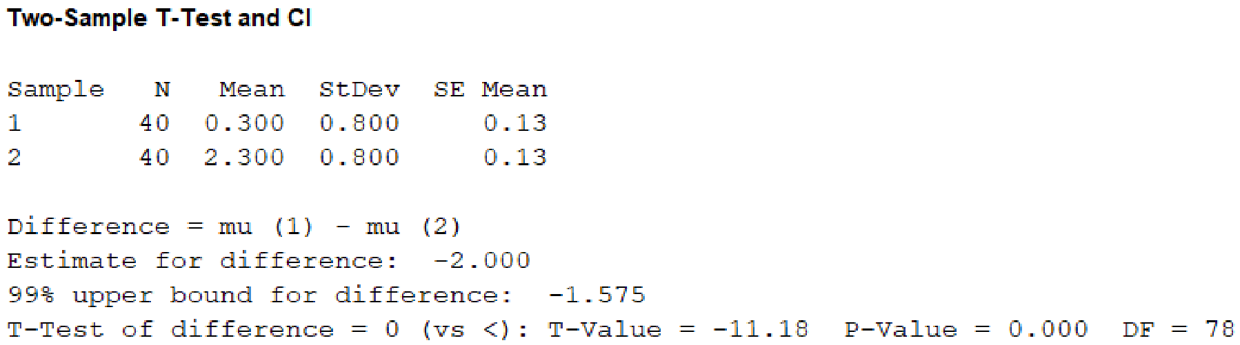
From the given MINITAB output, the value of test statistic is –11.18.
Step 8:
P-value:
From the MINITAB output, the P-value is 0.
Step 9:
Decision rule:
If the
Here, the
That is,
The decision is that the null hypothesis is rejected.
Conclusion:
Hence, there is sufficient evidence to conclude that the average number of miles per hour over the speed limit is smaller for male drivers with female passengers than it is for female drivers with male passengers.
c.
Comment on the effects of gender on teenagers driving with passengers.
c.
Explanation of Solution
Comment:
From the results, it is observed that the average speed limit for male and female drivers are greater with male passengers when compared to the female passengers. The average speed limit for male drivers are lesser with female passengers when compared to the female drivers with male passengers. The average speed limit for male drivers are greater with male passengers when compared to the female drivers with female passengers.
Want to see more full solutions like this?
Chapter 11 Solutions
Introduction to Statistics and Data Analysis


- ons 12. A sociologist hypothesizes that the crime rate is higher in areas with higher poverty rate and lower median income. She col- lects data on the crime rate (crimes per 100,000 residents), the poverty rate (in %), and the median income (in $1,000s) from 41 New England cities. A portion of the regression results is shown in the following table. Standard Coefficients error t stat p-value Intercept -301.62 549.71 -0.55 0.5864 Poverty 53.16 14.22 3.74 0.0006 Income 4.95 8.26 0.60 0.5526 a. b. Are the signs as expected on the slope coefficients? Predict the crime rate in an area with a poverty rate of 20% and a median income of $50,000. 3. Using data from 50 workarrow_forward2. The owner of several used-car dealerships believes that the selling price of a used car can best be predicted using the car's age. He uses data on the recent selling price (in $) and age of 20 used sedans to estimate Price = Po + B₁Age + ε. A portion of the regression results is shown in the accompanying table. Standard Coefficients Intercept 21187.94 Error 733.42 t Stat p-value 28.89 1.56E-16 Age -1208.25 128.95 -9.37 2.41E-08 a. What is the estimate for B₁? Interpret this value. b. What is the sample regression equation? C. Predict the selling price of a 5-year-old sedan.arrow_forwardian income of $50,000. erty rate of 13. Using data from 50 workers, a researcher estimates Wage = Bo+B,Education + B₂Experience + B3Age+e, where Wage is the hourly wage rate and Education, Experience, and Age are the years of higher education, the years of experience, and the age of the worker, respectively. A portion of the regression results is shown in the following table. ni ogolloo bash 1 Standard Coefficients error t stat p-value Intercept 7.87 4.09 1.93 0.0603 Education 1.44 0.34 4.24 0.0001 Experience 0.45 0.14 3.16 0.0028 Age -0.01 0.08 -0.14 0.8920 a. Interpret the estimated coefficients for Education and Experience. b. Predict the hourly wage rate for a 30-year-old worker with four years of higher education and three years of experience.arrow_forward
- 1. If a firm spends more on advertising, is it likely to increase sales? Data on annual sales (in $100,000s) and advertising expenditures (in $10,000s) were collected for 20 firms in order to estimate the model Sales = Po + B₁Advertising + ε. A portion of the regression results is shown in the accompanying table. Intercept Advertising Standard Coefficients Error t Stat p-value -7.42 1.46 -5.09 7.66E-05 0.42 0.05 8.70 7.26E-08 a. Interpret the estimated slope coefficient. b. What is the sample regression equation? C. Predict the sales for a firm that spends $500,000 annually on advertising.arrow_forwardCan you help me solve problem 38 with steps im stuck.arrow_forwardHow do the samples hold up to the efficiency test? What percentages of the samples pass or fail the test? What would be the likelihood of having the following specific number of efficiency test failures in the next 300 processors tested? 1 failures, 5 failures, 10 failures and 20 failures.arrow_forward
- The battery temperatures are a major concern for us. Can you analyze and describe the sample data? What are the average and median temperatures? How much variability is there in the temperatures? Is there anything that stands out? Our engineers’ assumption is that the temperature data is normally distributed. If that is the case, what would be the likelihood that the Safety Zone temperature will exceed 5.15 degrees? What is the probability that the Safety Zone temperature will be less than 4.65 degrees? What is the actual percentage of samples that exceed 5.25 degrees or are less than 4.75 degrees? Is the manufacturing process producing units with stable Safety Zone temperatures? Can you check if there are any apparent changes in the temperature pattern? Are there any outliers? A closer look at the Z-scores should help you in this regard.arrow_forwardNeed help pleasearrow_forwardPlease conduct a step by step of these statistical tests on separate sheets of Microsoft Excel. If the calculations in Microsoft Excel are incorrect, the null and alternative hypotheses, as well as the conclusions drawn from them, will be meaningless and will not receive any points. 4. One-Way ANOVA: Analyze the customer satisfaction scores across four different product categories to determine if there is a significant difference in means. (Hints: The null can be about maintaining status-quo or no difference among groups) H0 = H1=arrow_forward
- Please conduct a step by step of these statistical tests on separate sheets of Microsoft Excel. If the calculations in Microsoft Excel are incorrect, the null and alternative hypotheses, as well as the conclusions drawn from them, will be meaningless and will not receive any points 2. Two-Sample T-Test: Compare the average sales revenue of two different regions to determine if there is a significant difference. (Hints: The null can be about maintaining status-quo or no difference among groups; if alternative hypothesis is non-directional use the two-tailed p-value from excel file to make a decision about rejecting or not rejecting null) H0 = H1=arrow_forwardPlease conduct a step by step of these statistical tests on separate sheets of Microsoft Excel. If the calculations in Microsoft Excel are incorrect, the null and alternative hypotheses, as well as the conclusions drawn from them, will be meaningless and will not receive any points 3. Paired T-Test: A company implemented a training program to improve employee performance. To evaluate the effectiveness of the program, the company recorded the test scores of 25 employees before and after the training. Determine if the training program is effective in terms of scores of participants before and after the training. (Hints: The null can be about maintaining status-quo or no difference among groups; if alternative hypothesis is non-directional, use the two-tailed p-value from excel file to make a decision about rejecting or not rejecting the null) H0 = H1= Conclusion:arrow_forwardPlease conduct a step by step of these statistical tests on separate sheets of Microsoft Excel. If the calculations in Microsoft Excel are incorrect, the null and alternative hypotheses, as well as the conclusions drawn from them, will be meaningless and will not receive any points. The data for the following questions is provided in Microsoft Excel file on 4 separate sheets. Please conduct these statistical tests on separate sheets of Microsoft Excel. If the calculations in Microsoft Excel are incorrect, the null and alternative hypotheses, as well as the conclusions drawn from them, will be meaningless and will not receive any points. 1. One Sample T-Test: Determine whether the average satisfaction rating of customers for a product is significantly different from a hypothetical mean of 75. (Hints: The null can be about maintaining status-quo or no difference; If your alternative hypothesis is non-directional (e.g., μ≠75), you should use the two-tailed p-value from excel file to…arrow_forward
 Glencoe Algebra 1, Student Edition, 9780079039897...AlgebraISBN:9780079039897Author:CarterPublisher:McGraw Hill
 Big Ideas Math A Bridge To Success Algebra 1: Stu...AlgebraISBN:9781680331141Author:HOUGHTON MIFFLIN HARCOURTPublisher:Houghton Mifflin Harcourt
 College Algebra (MindTap Course List)AlgebraISBN:9781305652231Author:R. David Gustafson, Jeff HughesPublisher:Cengage Learning
 Holt Mcdougal Larson Pre-algebra: Student Edition...AlgebraISBN:9780547587776Author:HOLT MCDOUGALPublisher:HOLT MCDOUGAL