
Concept explainers
Videos
a.
To identify: The claim and state
a.
Answer to Problem 13E
The claim is that “the variance in the number of calories differs between the two brands”.
Null hypothesis:
Alternative hypothesis:
Explanation of Solution
Given info:
The data shows the areas (in square miles).
Justification:
Here, the claim is that “the variance in area is greater for eastern cities than for western cities”. This can be written as
b.
To find: The critical value for 5% level and 1% level.
b.
Answer to Problem 13E
The critical value at 5% level is 4.950 and the critical value at 1% level is 10.67.
Explanation of Solution
Calculation:
The degrees of freedom for numerator is,
The degrees of freedom for denominator is,
Software Procedure:
Step-by-step procedure to obtain the critical value using the MINITAB software:
- Choose Graph >
Probability Distribution Plot choose View Probability> OK. - From Distribution, choose F.
- Enter Numerator df as 6 and Denominator df as 5.
- Click the Shaded Area tab.
- Choose Probability value and Right Tail for the region of the curve to shade.
- Enter the Probability value as 0.05.
- Click OK.
Output using the MINITAB software is given below:
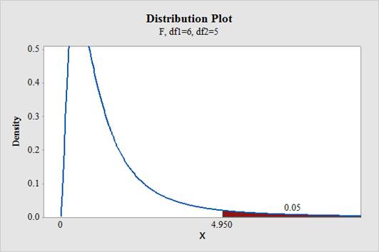
From the output, the critical value is 4.950.
Level of significance,
Software Procedure:
Step-by-step procedure to obtain the critical value using the MINITAB software:
- Choose Graph > Probability Distribution Plot choose View Probability> OK.
- From Distribution, choose F.
- Enter Numerator df as 6 and Denominator df as 5.
- Click the Shaded Area tab.
- Choose Probability value and Right Tail for the region of the curve to shade.
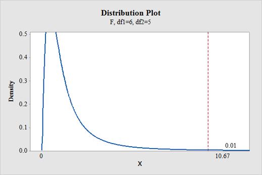
- Enter the Probability value as 0.01.
- Click OK.
Output using the MINITAB software is given below:
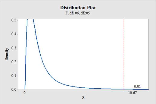
From the output, the critical value is 10.67.
c.
To find: The test value.
c.
Answer to Problem 13E
The test statistic value is 9.80.
Explanation of Solution
Calculation:
Software Procedure:
Step-by-step procedure to obtain the test value using the MINITAB software:
- Choose Stat > Basic Statistics >2 Variance.
- Choose Each sample is in its own column.
- In Sample 1, enter the column of Eastern.
- In Sample 2, enter the column of Western.
- Check Options; enter Confidence level as 95%.
- Choose greater than in alternative.
- Click OK.
Output using the MINITAB software is given below:
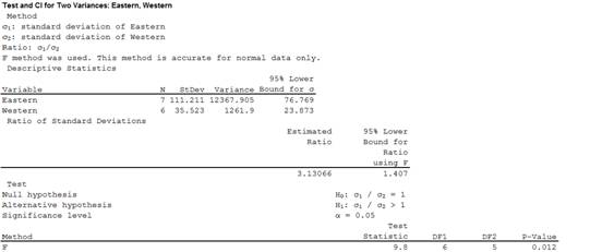
From the output, the test value is 9.80.
d.
To decide: Whether to reject or fail to reject the null hypothesis at a level of significance of
d.
Answer to Problem 13E
For 5% level, the decision is “reject the null hypothesis”.
For 1% level, the decision is “fail to reject the null hypothesis”.
Explanation of Solution
Calculation:
Software Procedure:
Step-by-step procedure to indicate the appropriate area and critical value using the MINITAB software:
- Choose Graph > Probability Distribution Plot choose View Probability> OK.
- From Distribution, choose F.
- Enter Numerator df as 8 and Denominator df as 8.
- Click the Shaded Area tab.
- Choose Probability value and Both Tail for the region of the curve to shade.
- Enter the Probability value as 0.05.
- Enter 9.80 under show reference lines at X values
- Click OK.
Output using the MINITAB software is given below:
From the output, it can be observed that the test statistic value falls in the rejection region. Therefore, the null hypothesis is rejected.
Software Procedure:
Step-by-step procedure to indicate the appropriate area and critical value using the MINITAB software:
- Choose Graph > Probability Distribution Plot choose View Probability> OK.
- From Distribution, choose F.
- Enter Numerator df as 8 and Denominator df as 8.
- Click the Shaded Area tab.
- Choose Probability value and Both Tail for the region of the curve to shade.
- Enter the Probability value as 0.01.
- Enter 9.80 under show reference lines at X values
- Click OK.
Output using the MINITAB software is given below:
From the output, it can be observed that the test statistic value do not falls in the rejection region. Therefore, the null hypothesis is not rejected.
e.
To summarize: The result.
e.
Answer to Problem 13E
The conclusion is that, there is enough evidence to support the claim that the variance in area is greater for eastern cities than for western cities at 5% level of significance.
The conclusion is that, there is no enough evidence to support the claim that the variance in area is greater for eastern cities than for western cities at 1% level of significance.
Explanation of Solution
Justification:
For 5% level:
From part (d), the null hypothesis is rejected. Thus, there is enough evidence to support the claim that the variance in area is greater for eastern cities than for western citiesat 5% level of significance.
For 1% level:
From part (d), the null hypothesis is not rejected. Thus, there is no enough evidence to support the claim that the variance in area is greater for eastern cities than for western cities at 1% level of significance.
Want to see more full solutions like this?
Chapter 9 Solutions
ELEMENTARY STATISTICS: STEP BY STEP- ALE


- In a company with 80 employees, 60 earn $10.00 per hour and 20 earn $13.00 per hour. Is this average hourly wage considered representative?arrow_forwardThe following is a list of questions answered correctly on an exam. Calculate the Measures of Central Tendency from the ungrouped data list. NUMBER OF QUESTIONS ANSWERED CORRECTLY ON AN APTITUDE EXAM 112 72 69 97 107 73 92 76 86 73 126 128 118 127 124 82 104 132 134 83 92 108 96 100 92 115 76 91 102 81 95 141 81 80 106 84 119 113 98 75 68 98 115 106 95 100 85 94 106 119arrow_forwardThe following ordered data list shows the data speeds for cell phones used by a telephone company at an airport: A. Calculate the Measures of Central Tendency using the table in point B. B. Are there differences in the measurements obtained in A and C? Why (give at least one justified reason)? 0.8 1.4 1.8 1.9 3.2 3.6 4.5 4.5 4.6 6.2 6.5 7.7 7.9 9.9 10.2 10.3 10.9 11.1 11.1 11.6 11.8 12.0 13.1 13.5 13.7 14.1 14.2 14.7 15.0 15.1 15.5 15.8 16.0 17.5 18.2 20.2 21.1 21.5 22.2 22.4 23.1 24.5 25.7 28.5 34.6 38.5 43.0 55.6 71.3 77.8arrow_forward
- In a company with 80 employees, 60 earn $10.00 per hour and 20 earn $13.00 per hour. a) Determine the average hourly wage. b) In part a), is the same answer obtained if the 60 employees have an average wage of $10.00 per hour? Prove your answer.arrow_forwardThe following ordered data list shows the data speeds for cell phones used by a telephone company at an airport: A. Calculate the Measures of Central Tendency from the ungrouped data list. B. Group the data in an appropriate frequency table. 0.8 1.4 1.8 1.9 3.2 3.6 4.5 4.5 4.6 6.2 6.5 7.7 7.9 9.9 10.2 10.3 10.9 11.1 11.1 11.6 11.8 12.0 13.1 13.5 13.7 14.1 14.2 14.7 15.0 15.1 15.5 15.8 16.0 17.5 18.2 20.2 21.1 21.5 22.2 22.4 23.1 24.5 25.7 28.5 34.6 38.5 43.0 55.6 71.3 77.8arrow_forwardBusinessarrow_forward
- https://www.hawkeslearning.com/Statistics/dbs2/datasets.htmlarrow_forwardNC Current Students - North Ce X | NC Canvas Login Links - North ( X Final Exam Comprehensive x Cengage Learning x WASTAT - Final Exam - STAT → C webassign.net/web/Student/Assignment-Responses/submit?dep=36055360&tags=autosave#question3659890_9 Part (b) Draw a scatter plot of the ordered pairs. N Life Expectancy Life Expectancy 80 70 600 50 40 30 20 10 Year of 1950 1970 1990 2010 Birth O Life Expectancy Part (c) 800 70 60 50 40 30 20 10 1950 1970 1990 W ALT 林 $ # 4 R J7 Year of 2010 Birth F6 4+ 80 70 60 50 40 30 20 10 Year of 1950 1970 1990 2010 Birth Life Expectancy Ox 800 70 60 50 40 30 20 10 Year of 1950 1970 1990 2010 Birth hp P.B. KA & 7 80 % 5 H A B F10 711 N M K 744 PRT SC ALT CTRLarrow_forwardHarvard University California Institute of Technology Massachusetts Institute of Technology Stanford University Princeton University University of Cambridge University of Oxford University of California, Berkeley Imperial College London Yale University University of California, Los Angeles University of Chicago Johns Hopkins University Cornell University ETH Zurich University of Michigan University of Toronto Columbia University University of Pennsylvania Carnegie Mellon University University of Hong Kong University College London University of Washington Duke University Northwestern University University of Tokyo Georgia Institute of Technology Pohang University of Science and Technology University of California, Santa Barbara University of British Columbia University of North Carolina at Chapel Hill University of California, San Diego University of Illinois at Urbana-Champaign National University of Singapore McGill…arrow_forward
- Name Harvard University California Institute of Technology Massachusetts Institute of Technology Stanford University Princeton University University of Cambridge University of Oxford University of California, Berkeley Imperial College London Yale University University of California, Los Angeles University of Chicago Johns Hopkins University Cornell University ETH Zurich University of Michigan University of Toronto Columbia University University of Pennsylvania Carnegie Mellon University University of Hong Kong University College London University of Washington Duke University Northwestern University University of Tokyo Georgia Institute of Technology Pohang University of Science and Technology University of California, Santa Barbara University of British Columbia University of North Carolina at Chapel Hill University of California, San Diego University of Illinois at Urbana-Champaign National University of Singapore…arrow_forwardA company found that the daily sales revenue of its flagship product follows a normal distribution with a mean of $4500 and a standard deviation of $450. The company defines a "high-sales day" that is, any day with sales exceeding $4800. please provide a step by step on how to get the answers in excel Q: What percentage of days can the company expect to have "high-sales days" or sales greater than $4800? Q: What is the sales revenue threshold for the bottom 10% of days? (please note that 10% refers to the probability/area under bell curve towards the lower tail of bell curve) Provide answers in the yellow cellsarrow_forwardFind the critical value for a left-tailed test using the F distribution with a 0.025, degrees of freedom in the numerator=12, and degrees of freedom in the denominator = 50. A portion of the table of critical values of the F-distribution is provided. Click the icon to view the partial table of critical values of the F-distribution. What is the critical value? (Round to two decimal places as needed.)arrow_forward
 Glencoe Algebra 1, Student Edition, 9780079039897...AlgebraISBN:9780079039897Author:CarterPublisher:McGraw Hill
 College Algebra (MindTap Course List)AlgebraISBN:9781305652231Author:R. David Gustafson, Jeff HughesPublisher:Cengage Learning
 Holt Mcdougal Larson Pre-algebra: Student Edition...AlgebraISBN:9780547587776Author:HOLT MCDOUGALPublisher:HOLT MCDOUGAL
