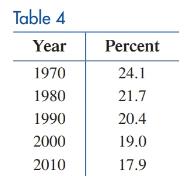
The population center of the 48 contiguous states of the United States is the point where a flat, rigid map of the contiguous states would balance if the location of each person was represented on the map by a weight of equal measure. In 1790, the population center was 23 miles east of Baltimore, Maryland. By 1990, the center had shifted about 800 miles west and 100 miles south to a point in southeast Missouri. To study this shifting population, the U.S. Census Bureau divides the states into four regions as shown in the figure. Problems 69 and 70 deal with population shifts among these regions. Population shifts. Table 3 gives the percentage of the U.S. population living in the south region during the indicated years. The following transition matrix P is proposed as a model for the data, where N represents the population that lives in the south region: Next decade N N ′ Current decade N N ′ .61 .39 .09 .91 = P (A) Let S 0 = .241 .759 and find S 1 , S 2 , S 3 , and S 4 . Compute the matrices exactly and then round entries to three decimal places. (B) Construct a new table comparing the results from part (A) with the data in Table 4. (C) According to this transition matrix, what percentage of the population will live in the northeast region in the long run?
The population center of the 48 contiguous states of the United States is the point where a flat, rigid map of the contiguous states would balance if the location of each person was represented on the map by a weight of equal measure. In 1790, the population center was 23 miles east of Baltimore, Maryland. By 1990, the center had shifted about 800 miles west and 100 miles south to a point in southeast Missouri. To study this shifting population, the U.S. Census Bureau divides the states into four regions as shown in the figure. Problems 69 and 70 deal with population shifts among these regions. Population shifts. Table 3 gives the percentage of the U.S. population living in the south region during the indicated years. The following transition matrix P is proposed as a model for the data, where N represents the population that lives in the south region: Next decade N N ′ Current decade N N ′ .61 .39 .09 .91 = P (A) Let S 0 = .241 .759 and find S 1 , S 2 , S 3 , and S 4 . Compute the matrices exactly and then round entries to three decimal places. (B) Construct a new table comparing the results from part (A) with the data in Table 4. (C) According to this transition matrix, what percentage of the population will live in the northeast region in the long run?
Solution Summary: The author explains that the first transition matrix S_1 is given by, lnext decadeN ' P=
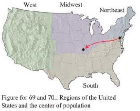
The population center of the 48 contiguous states of the United States is the point where a flat, rigid map of the contiguous states would balance if the location of each person was represented on the map by a weight of equal measure. In 1790, the population center was 23 miles east of Baltimore, Maryland. By 1990, the center had shifted about 800 miles west and 100 miles south to a point in southeast Missouri. To study this shifting population, the U.S. Census Bureau divides the states into four regions as shown in the figure. Problems 69 and 70 deal with population shifts among these regions.
Population shifts. Table 3 gives the percentage of the U.S. population living in the south region during the indicated years.
The following transition matrix
P
is proposed as a model for the data, where
N
represents the population that lives in the south region:
Next decade
N
N
′
Current
decade
N
N
′
.61
.39
.09
.91
=
P
(A) Let
S
0
=
.241
.759
and find
S
1
,
S
2
,
S
3
, and
S
4
. Compute the matrices exactly and then round entries to three decimal places.
(B) Construct a new table comparing the results from part (A) with the data in Table 4.
(C) According to this transition matrix, what percentage of the population will live in the northeast region in the long run?
Topic 2
Evaluate S
x
dx, using u-substitution. Then find the integral using
1-x2
trigonometric substitution. Discuss the results!
Topic 3
Explain what an elementary anti-derivative is. Then consider the following
ex
integrals: fed dx
x
1
Sdx
In x
Joseph Liouville proved that the first integral does not have an elementary anti-
derivative Use this fact to prove that the second integral does not have an
elementary anti-derivative. (hint: use an appropriate u-substitution!)
1. Given the vector field F(x, y, z) = -xi, verify the relation
1
V.F(0,0,0) = lim
0+ volume inside Se
ff F• Nds
SE
where SE is the surface enclosing a cube centred at the origin and having edges of length 2€. Then,
determine if the origin is sink or source.
4
3
2
-5 4-3 -2 -1
1 2 3 4 5
12
23
-4
The function graphed above is:
Increasing on the interval(s)
Decreasing on the interval(s)
Chapter 9 Solutions
Pearson eText for Finite Mathematics for Business, Economics, Life Sciences, and Social Sciences -- Instant Access (Pearson+)
Need a deep-dive on the concept behind this application? Look no further. Learn more about this topic, subject and related others by exploring similar questions and additional content below.


 Algebra: Structure And Method, Book 1AlgebraISBN:9780395977224Author:Richard G. Brown, Mary P. Dolciani, Robert H. Sorgenfrey, William L. ColePublisher:McDougal Littell
 Glencoe Algebra 1, Student Edition, 9780079039897...AlgebraISBN:9780079039897Author:CarterPublisher:McGraw Hill
 Mathematics For Machine TechnologyAdvanced MathISBN:9781337798310Author:Peterson, John.Publisher:Cengage Learning,
 Holt Mcdougal Larson Pre-algebra: Student Edition...AlgebraISBN:9780547587776Author:HOLT MCDOUGALPublisher:HOLT MCDOUGAL