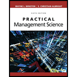
Practical Management Science
6th Edition
ISBN: 9781337406659
Author: WINSTON, Wayne L.
Publisher: Cengage,
expand_more
expand_more
format_list_bulleted
Concept explainers
Question
Chapter 8.6, Problem 12P
Summary Introduction
To determine: The evolutionary solver to fit a pearl and Gompertz curve.
Introduction: The variation between the present value of the
Expert Solution & Answer
Want to see the full answer?
Check out a sample textbook solution
Students have asked these similar questions
what is the arithmetic average annual return per year?
Describe a simple sales information system for an online store, including its products, branches, and its appraisal, so that it captures the attention of an average person without a university degree or a particular career, and develop a report about it.
Note: A waiting line model solver computer package is needed to answer these questions.
The Kolkmeyer Manufacturing Company uses a group of six identical machines, each of which operates an average of 23 hours between breakdowns. With randomly occurring breakdowns, the Poisson probability distribution is used to describe the machine breakdown
arrival process. One person from the maintenance department provides the single-server repair service for the six machines.
Management is now considering adding two machines to its manufacturing operation. This addition will bring the number of machines to eight. The president of Kolkmeyer asked for a study of the need to add a second employee to the repair operation. The service rate
for each individual assigned to the repair operation is 0.40 machines per hour.
(a) Compute the operating characteristics if the company retains the single-employee repair operation. (Round your answers to four decimal places. Report time in hours.)
La
=
L =
Wa
W =
h…
Chapter 8 Solutions
Practical Management Science
Ch. 8.3 - Prob. 1PCh. 8.3 - Prob. 2PCh. 8.4 - Prob. 3PCh. 8.4 - Prob. 4PCh. 8.4 - Prob. 5PCh. 8.5 - Prob. 6PCh. 8.5 - Prob. 7PCh. 8.5 - In the lawn mower production problem in Example...Ch. 8.6 - Prob. 9PCh. 8.6 - Prob. 10P
Ch. 8.6 - Prob. 11PCh. 8.6 - Prob. 12PCh. 8.7 - Prob. 13PCh. 8.7 - Prob. 14PCh. 8.8 - Prob. 15PCh. 8.8 - Prob. 16PCh. 8.8 - Prob. 17PCh. 8.8 - Prob. 18PCh. 8.8 - Prob. 19PCh. 8 - Prob. 20PCh. 8 - Prob. 21PCh. 8 - Prob. 22PCh. 8 - Prob. 23PCh. 8 - Prob. 24PCh. 8 - Prob. 25PCh. 8 - Prob. 26PCh. 8 - Prob. 27PCh. 8 - Prob. 28PCh. 8 - Prob. 29PCh. 8 - Prob. 30PCh. 8 - Prob. 31PCh. 8 - Prob. 32PCh. 8 - Prob. 33PCh. 8 - Prob. 34PCh. 8 - Prob. 35PCh. 8 - Prob. 36PCh. 8 - Prob. 37PCh. 8 - Prob. 38PCh. 8 - Prob. 39PCh. 8 - Prob. 1CCh. 8 - Prob. 2C
Knowledge Booster
Learn more about
Need a deep-dive on the concept behind this application? Look no further. Learn more about this topic, operations-management and related others by exploring similar questions and additional content below.Similar questions
- Burger Dome sells hamburgers, cheeseburgers, french fries, soft drinks, and milk shakes, as well as a limited number of specialty items and dessert selections. Although Burger Dome would like to serve each customer immediately, at times more customers arrive than can be handled by the Burger Dome food service staff. Thus, customers wait in line to place and receive their orders. Burger Dome analyzed data on customer arrivals and concluded that the arrival rate is 40 customers per hour. Burger Dome also studied the order-filling process and found that a single employee can process an average of 56 customer orders per hour. Burger Dome is concerned that the methods currently used to serve customers are resulting in excessive waiting times and a possible loss of sales. Management wants to conduct a waiting line study to help determine the best approach to reduce waiting times and improve service. Suppose Burger Dome establishes two servers but arranges the restaurant layout so that an…arrow_forwardAgan Interior Design provides home and office decorating assistance to its customers. In normal operation, an average of 2.6 customers arrive each hour. One design consultant is available to answer customer questions and make product recommendations. The consultant averages 10 minutes with each customer. (a) Compute the operating characteristics of the customer waiting line, assuming Poisson arrivals and exponential service times. (Round your answers to four decimal places. Report time in hours.) λ= μ = = L = Wa W = P. W h (b) Service goals dictate that an arriving customer should not wait for service more than an average of 5 minutes. Is this goal being met? (Round your answer to one decimal place.) W₁ (in minutes) = min, which is ---Select--- than the desired wait time, so the goal ---Select--- met. What action do you recommend? (Select all that apply.) Hire another consultant. Increase the hours of operation. Decrease the mean service rate. Increase the mean service rate. There is…arrow_forwardCommunication Tips (2015) Tactful bragging Respond to the question "So, what do you do?" Whether you are student or have a job/internship, how can you tactfully brag in your answer to this question? Use the three elements from the video (listed below) when crafting your brag statement: Focus on results vs title Process vs job description Loop back to listener Example of an instructor's brag statement: "I help hundreds of students each semester to connect with one another, develop communication skills and prepare for upcoming interviews. Through improv games we explore presence, flexibility, and storytelling. How have your networking experiences on campus been so far?"arrow_forward
- Accounting problemarrow_forwardGovernment's new plan to shift cargo from roads back to rail 26TH JANUARY 2024 Government is seeking to finalise a plan aimed at improving its rail network and move cargo away from a billion rand per day to its logistics crises, government has said an urgentturnaround is needed to improve its 31 000km locomotive network as more and more cargo moves from rail to trucks. The Department of Transport (DoT) hosted a discussion with industry stakeholders regarding the Freight Road to Rail Migration Plan on Thursday - the latest development in the wake of President Cyril Ramphosa forming the National Logistics Crisis Committee last year. Transnet, the South African National Roads Agency (Sanral) and private sector companies were all in attendance. The Freight Road to Rail Migration Plan is part of government's strategies to improve the country's ongoing logistics crises. In October last year, the government unveiled its Freight Logistics Roadmap to improve the ports and rail networks and…arrow_forwardAssess what led to such logistical inefficiencies / collapse of a previously world class freight networkarrow_forward
- Which of the following statements concerning the evaluation of training programs is true? Most companies thoroughly evaluate the return on investment of their training programs It is relatively easy to establish a control group and a treatment group for evaluation Results level of evaluation measures how well participants liked the program Behavior level criteria measure whether skills learned in training result in behavior changes back on the jobarrow_forwardEligibility testing is an disparate impact validation method none of the above a method to validate promotions and progressive discipline activity a test an employee administers to ensure that the potential employee is capable and qualified to perform the requirements of the positionarrow_forwardA no-strike pledge by a union in a collective bargaining agreement is given in return for management’s agreement to: a grievance procedure a union shop a wage increase a fringe benefit increase binding arbitration of grievancesarrow_forward
- Which is the major OD technique that is used for increasing the communication, cooperation, and cohesiveness of work units? Leadership analysis Developing objectives Groupthink Strategic Planning team Buildingarrow_forwardAn American multinational firm usually is less than fully successful in adapting itself to local practices in each country because: American managers are often ignorant of local conditions None of the above management direction may be centralized in the home office All of the above Foreign subsidiaries often have American managersarrow_forwardWhen salary increases are based on inputs, or performance, companies are following: agency theory equality theory equity theory compliance theory need theoryarrow_forward
arrow_back_ios
SEE MORE QUESTIONS
arrow_forward_ios
Recommended textbooks for you
 Practical Management ScienceOperations ManagementISBN:9781337406659Author:WINSTON, Wayne L.Publisher:Cengage,

Practical Management Science
Operations Management
ISBN:9781337406659
Author:WINSTON, Wayne L.
Publisher:Cengage,
Inventory Management | Concepts, Examples and Solved Problems; Author: Dr. Bharatendra Rai;https://www.youtube.com/watch?v=2n9NLZTIlz8;License: Standard YouTube License, CC-BY