
Statistics for Engineers and Scientists
4th Edition
ISBN: 9780073401331
Author: William Navidi Prof.
Publisher: McGraw-Hill Education
expand_more
expand_more
format_list_bulleted
Videos
Textbook Question
Chapter 8.2, Problem 1E
In an experiment to determine factors related to weld toughness, the Charpy V-notch impact toughness in ft·lb (y) was measured for 22 welds at 0°C, along with the lateral expansion at the notch in % (x1), and the brittle fracture surface in % (x2). The data are presented in the following table.
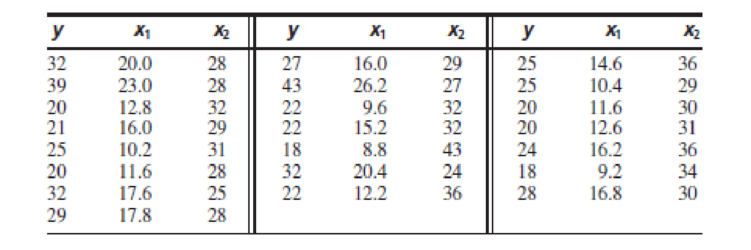
- a. Fit the model y = β0 + β1x1 + ε. For each coefficient, test the null hypothesis that it is equal to 0.
- b. Fit the model y = β0 + β1x2 + ε. For each coefficient, test the null hypothesis that it is equal to 0.
- c. Fit the model y = β0 + β1x1 + β2x2 + ε. For each coefficient, test the null hypothesis that it is equal to 0.
- d. Which of the models in parts (a) through (c) is the best of the three? Why do you think so?
Expert Solution & Answer
Want to see the full answer?
Check out a sample textbook solution
Students have asked these similar questions
0|0|0|0
-
Consider the time series X₁ and Y₁ = (I – B)² (I – B³)Xt. What transformations were
performed on Xt to obtain Yt?
seasonal difference of order 2
simple difference of order 5
seasonal difference of order 1
seasonal difference of order 5
simple difference of order 2
Calculate the 90% confidence interval for the population mean difference using the data in the attached image. I need to see where I went wrong.
Microsoft Excel snapshot for random sampling: Also note the formula used for the last
column
02
x✓ fx =INDEX(5852:58551, RANK(C2, $C$2:$C$51))
A
B
1
No.
States
2
1
ALABAMA
Rand No.
0.925957526
3
2
ALASKA
0.372999976
4
3
ARIZONA
0.941323044
5
4 ARKANSAS
0.071266381
Random Sample
CALIFORNIA
NORTH CAROLINA
ARKANSAS
WASHINGTON
G7
Microsoft Excel snapshot for systematic sampling:
xfx INDEX(SD52:50551, F7)
A
B
E
F
G
1
No.
States
Rand No. Random Sample
population
50
2
1 ALABAMA
0.5296685 NEW HAMPSHIRE
sample
10
3
2 ALASKA
0.4493186 OKLAHOMA
k
5
4
3 ARIZONA
0.707914 KANSAS
5
4 ARKANSAS 0.4831379 NORTH DAKOTA
6
5 CALIFORNIA 0.7277162 INDIANA
Random Sample
Sample Name
7
6 COLORADO 0.5865002 MISSISSIPPI
8
7:ONNECTICU 0.7640596 ILLINOIS
9
8 DELAWARE 0.5783029 MISSOURI
525
10
15
INDIANA
MARYLAND
COLORADO
Chapter 8 Solutions
Statistics for Engineers and Scientists
Ch. 8.1 - In an experiment to determine the factors...Ch. 8.1 - Prob. 2ECh. 8.1 - Prob. 3ECh. 8.1 - The article Application of Analysis of Variance to...Ch. 8.1 - Prob. 5ECh. 8.1 - Prob. 6ECh. 8.1 - Prob. 7ECh. 8.1 - Refer to Exercise 7. a. Find a 95% confidence...Ch. 8.1 - In a study of the lung function of children, the...Ch. 8.1 - Prob. 10E
Ch. 8.1 - Prob. 11ECh. 8.1 - The following MINITAB output is for a multiple...Ch. 8.1 - Prob. 13ECh. 8.1 - Prob. 14ECh. 8.1 - Prob. 15ECh. 8.1 - The following data were collected in an experiment...Ch. 8.1 - The November 24, 2001, issue of The Economist...Ch. 8.1 - The article Multiple Linear Regression for Lake...Ch. 8.1 - Prob. 19ECh. 8.2 - In an experiment to determine factors related to...Ch. 8.2 - In a laboratory test of a new engine design, the...Ch. 8.2 - In a laboratory test of a new engine design, the...Ch. 8.2 - The article Influence of Freezing Temperature on...Ch. 8.2 - The article Influence of Freezing Temperature on...Ch. 8.2 - The article Influence of Freezing Temperature on...Ch. 8.3 - True or false: a. For any set of data, there is...Ch. 8.3 - The article Experimental Design Approach for the...Ch. 8.3 - Prob. 3ECh. 8.3 - An engineer measures a dependent variable y and...Ch. 8.3 - Prob. 5ECh. 8.3 - The following MINITAB output is for a best subsets...Ch. 8.3 - Prob. 7ECh. 8.3 - Prob. 8ECh. 8.3 - (Continues Exercise 7 in Section 8.1.) To try to...Ch. 8.3 - Prob. 10ECh. 8.3 - Prob. 11ECh. 8.3 - Prob. 12ECh. 8.3 - The article Ultimate Load Analysis of Plate...Ch. 8.3 - Prob. 14ECh. 8.3 - Prob. 15ECh. 8.3 - Prob. 16ECh. 8.3 - The article Modeling Resilient Modulus and...Ch. 8.3 - The article Models for Assessing Hoisting Times of...Ch. 8 - The article Advances in Oxygen Equivalence...Ch. 8 - Prob. 2SECh. 8 - Prob. 3SECh. 8 - Prob. 4SECh. 8 - In a simulation of 30 mobile computer networks,...Ch. 8 - The data in Table SE6 (page 649) consist of yield...Ch. 8 - Prob. 7SECh. 8 - Prob. 8SECh. 8 - Refer to Exercise 2 in Section 8.2. a. Using each...Ch. 8 - Prob. 10SECh. 8 - The data presented in the following table give the...Ch. 8 - The article Enthalpies and Entropies of Transfer...Ch. 8 - Prob. 13SECh. 8 - Prob. 14SECh. 8 - The article Measurements of the Thermal...Ch. 8 - The article Electrical Impedance Variation with...Ch. 8 - The article Groundwater Electromagnetic Imaging in...Ch. 8 - Prob. 18SECh. 8 - Prob. 19SECh. 8 - Prob. 20SECh. 8 - Prob. 21SECh. 8 - Prob. 22SECh. 8 - The article Estimating Resource Requirements at...Ch. 8 - Prob. 24SE
Additional Math Textbook Solutions
Find more solutions based on key concepts
Evaluate the integrals in Exercises 1–46.
1.
University Calculus: Early Transcendentals (4th Edition)
Empirical versus Theoretical A Monopoly player claims that the probability of getting a 4 when rolling a six-si...
Introductory Statistics
1. How is a sample related to a population?
Elementary Statistics: Picturing the World (7th Edition)
Fill in each blank so that the resulting statement is true.
1. The degree of the polynomial function is _____....
Algebra and Trigonometry (6th Edition)
Provide an example of a qualitative variable and an example of a quantitative variable.
Elementary Statistics ( 3rd International Edition ) Isbn:9781260092561
(a) Make a stem-and-leaf plot for these 24 observations on the number of customers who used a down-town CitiBan...
APPLIED STAT.IN BUS.+ECONOMICS
Knowledge Booster


Learn more about
Need a deep-dive on the concept behind this application? Look no further. Learn more about this topic, statistics and related others by exploring similar questions and additional content below.Similar questions
- Suppose the Internal Revenue Service reported that the mean tax refund for the year 2022 was $3401. Assume the standard deviation is $82.5 and that the amounts refunded follow a normal probability distribution. Solve the following three parts? (For the answer to question 14, 15, and 16, start with making a bell curve. Identify on the bell curve where is mean, X, and area(s) to be determined. 1.What percent of the refunds are more than $3,500? 2. What percent of the refunds are more than $3500 but less than $3579? 3. What percent of the refunds are more than $3325 but less than $3579?arrow_forwardA normal distribution has a mean of 50 and a standard deviation of 4. Solve the following three parts? 1. Compute the probability of a value between 44.0 and 55.0. (The question requires finding probability value between 44 and 55. Solve it in 3 steps. In the first step, use the above formula and x = 44, calculate probability value. In the second step repeat the first step with the only difference that x=55. In the third step, subtract the answer of the first part from the answer of the second part.) 2. Compute the probability of a value greater than 55.0. Use the same formula, x=55 and subtract the answer from 1. 3. Compute the probability of a value between 52.0 and 55.0. (The question requires finding probability value between 52 and 55. Solve it in 3 steps. In the first step, use the above formula and x = 52, calculate probability value. In the second step repeat the first step with the only difference that x=55. In the third step, subtract the answer of the first part from the…arrow_forwardIf a uniform distribution is defined over the interval from 6 to 10, then answer the followings: What is the mean of this uniform distribution? Show that the probability of any value between 6 and 10 is equal to 1.0 Find the probability of a value more than 7. Find the probability of a value between 7 and 9. The closing price of Schnur Sporting Goods Inc. common stock is uniformly distributed between $20 and $30 per share. What is the probability that the stock price will be: More than $27? Less than or equal to $24? The April rainfall in Flagstaff, Arizona, follows a uniform distribution between 0.5 and 3.00 inches. What is the mean amount of rainfall for the month? What is the probability of less than an inch of rain for the month? What is the probability of exactly 1.00 inch of rain? What is the probability of more than 1.50 inches of rain for the month? The best way to solve this problem is begin by a step by step creating a chart. Clearly mark the range, identifying the…arrow_forward
- Client 1 Weight before diet (pounds) Weight after diet (pounds) 128 120 2 131 123 3 140 141 4 178 170 5 121 118 6 136 136 7 118 121 8 136 127arrow_forwardClient 1 Weight before diet (pounds) Weight after diet (pounds) 128 120 2 131 123 3 140 141 4 178 170 5 121 118 6 136 136 7 118 121 8 136 127 a) Determine the mean change in patient weight from before to after the diet (after – before). What is the 95% confidence interval of this mean difference?arrow_forwardIn order to find probability, you can use this formula in Microsoft Excel: The best way to understand and solve these problems is by first drawing a bell curve and marking key points such as x, the mean, and the areas of interest. Once marked on the bell curve, figure out what calculations are needed to find the area of interest. =NORM.DIST(x, Mean, Standard Dev., TRUE). When the question mentions “greater than” you may have to subtract your answer from 1. When the question mentions “between (two values)”, you need to do separate calculation for both values and then subtract their results to get the answer. 1. Compute the probability of a value between 44.0 and 55.0. (The question requires finding probability value between 44 and 55. Solve it in 3 steps. In the first step, use the above formula and x = 44, calculate probability value. In the second step repeat the first step with the only difference that x=55. In the third step, subtract the answer of the first part from the…arrow_forward
- If a uniform distribution is defined over the interval from 6 to 10, then answer the followings: What is the mean of this uniform distribution? Show that the probability of any value between 6 and 10 is equal to 1.0 Find the probability of a value more than 7. Find the probability of a value between 7 and 9. The closing price of Schnur Sporting Goods Inc. common stock is uniformly distributed between $20 and $30 per share. What is the probability that the stock price will be: More than $27? Less than or equal to $24? The April rainfall in Flagstaff, Arizona, follows a uniform distribution between 0.5 and 3.00 inches. What is the mean amount of rainfall for the month? What is the probability of less than an inch of rain for the month? What is the probability of exactly 1.00 inch of rain? What is the probability of more than 1.50 inches of rain for the month? The best way to solve this problem is begin by creating a chart. Clearly mark the range, identifying the lower and upper…arrow_forwardProblem 1: The mean hourly pay of an American Airlines flight attendant is normally distributed with a mean of 40 per hour and a standard deviation of 3.00 per hour. What is the probability that the hourly pay of a randomly selected flight attendant is: Between the mean and $45 per hour? More than $45 per hour? Less than $32 per hour? Problem 2: The mean of a normal probability distribution is 400 pounds. The standard deviation is 10 pounds. What is the area between 415 pounds and the mean of 400 pounds? What is the area between the mean and 395 pounds? What is the probability of randomly selecting a value less than 395 pounds? Problem 3: In New York State, the mean salary for high school teachers in 2022 was 81,410 with a standard deviation of 9,500. Only Alaska’s mean salary was higher. Assume New York’s state salaries follow a normal distribution. What percent of New York State high school teachers earn between 70,000 and 75,000? What percent of New York State high school…arrow_forwardPls help asaparrow_forward
- Solve the following LP problem using the Extreme Point Theorem: Subject to: Maximize Z-6+4y 2+y≤8 2x + y ≤10 2,y20 Solve it using the graphical method. Guidelines for preparation for the teacher's questions: Understand the basics of Linear Programming (LP) 1. Know how to formulate an LP model. 2. Be able to identify decision variables, objective functions, and constraints. Be comfortable with graphical solutions 3. Know how to plot feasible regions and find extreme points. 4. Understand how constraints affect the solution space. Understand the Extreme Point Theorem 5. Know why solutions always occur at extreme points. 6. Be able to explain how optimization changes with different constraints. Think about real-world implications 7. Consider how removing or modifying constraints affects the solution. 8. Be prepared to explain why LP problems are used in business, economics, and operations research.arrow_forwardged the variance for group 1) Different groups of male stalk-eyed flies were raised on different diets: a high nutrient corn diet vs. a low nutrient cotton wool diet. Investigators wanted to see if diet quality influenced eye-stalk length. They obtained the following data: d Diet Sample Mean Eye-stalk Length Variance in Eye-stalk d size, n (mm) Length (mm²) Corn (group 1) 21 2.05 0.0558 Cotton (group 2) 24 1.54 0.0812 =205-1.54-05T a) Construct a 95% confidence interval for the difference in mean eye-stalk length between the two diets (e.g., use group 1 - group 2).arrow_forwardAn article in Business Week discussed the large spread between the federal funds rate and the average credit card rate. The table below is a frequency distribution of the credit card rate charged by the top 100 issuers. Credit Card Rates Credit Card Rate Frequency 18% -23% 19 17% -17.9% 16 16% -16.9% 31 15% -15.9% 26 14% -14.9% Copy Data 8 Step 1 of 2: Calculate the average credit card rate charged by the top 100 issuers based on the frequency distribution. Round your answer to two decimal places.arrow_forward
arrow_back_ios
SEE MORE QUESTIONS
arrow_forward_ios
Recommended textbooks for you
 Algebra & Trigonometry with Analytic GeometryAlgebraISBN:9781133382119Author:SwokowskiPublisher:Cengage
Algebra & Trigonometry with Analytic Geometry
Algebra
ISBN:9781133382119
Author:Swokowski
Publisher:Cengage
Type I and II Errors, Power, Effect Size, Significance and Power Analysis in Quantitative Research; Author: NurseKillam;https://www.youtube.com/watch?v=OWn3Ko1WYTA;License: Standard YouTube License, CC-BY