
Concept explainers
Videos
a.
Find the 95% confidence interval for the slope of Manganese.
a.
Answer to Problem 2E
The 95% confidence interval for the slope of Manganese is
Explanation of Solution
Given info:
The data represents the MINITAB output of the regression model
Calculation:
Multiple linear regression model:
A multiple linear regression model is given as
The ‘Coefficient’ column of the regression analysis MINITAB output gives the slopes corresponding to the respective variables stored in the column ‘Predictor’.
Let
From the accompanying MINITAB output, the slope coefficient of Manganese is
Confidence interval:
The general formula for the confidence interval for the slope of the regression line is,
Where,
From the accompanying MINITAB output, the estimate of error standard deviation of slope coefficient of Manganese is
Critical value:
For 95% confidence level,
Degrees of freedom:
The number of plates that are sampled is
The degrees of freedom is,
From Table A.5 of the t- distribution in Appendix A, the critical value corresponding to the right tail area 0.025 and 17 degrees of freedom is 2.110.
Thus, the critical value is
The 95% confidence interval is,
Thus, the 95% confidence interval for the slope of Manganese is
Interpretation:
There is 95% confident that the average change in the tensile strength associated with 1 ppt increase in manganese lies between
b.
Find the 99% confidence interval for the slope of Thickness.
b.
Answer to Problem 2E
The 99% confidence interval for the slope of Thickness is
Explanation of Solution
Calculation:
From the accompanying MINITAB output, the slope coefficient of Thickness is
Confidence interval:
The general formula for the confidence interval for the slope of the regression line is,
Where,
From the accompanying MINITAB output, the estimate of error standard deviation of slope coefficient of Thickness is
Critical value:
For 99% confidence level,
Degrees of freedom:
The number of plates that are sampled is
The degrees of freedom is,
From Table A.5 of the t- distribution in Appendix A, the critical value corresponding to the right tail area 0.005 and 17 degrees of freedom is 2.898.
Thus, the critical value is
The 95% confidence interval is,
Thus, the 99% confidence interval for the slope of Thickness is
Interpretation:
There is 99% confident that the average change in the tensile strength associated with 1 ppt increase in Thickness lies between
c.
Test whether there is enough evidence to conclude that
c.
Answer to Problem 2E
There is no sufficient evidence to conclude that
Explanation of Solution
Calculation:
From the accompanying MINITAB output, the slope coefficient of Manganese is
Here, the claim is that
The test hypotheses are given below:
Null hypothesis:
That is, 1 ppt increase in manganese tends to at most
Alternative hypothesis:
That is, increase in the true average of tensile strength due to 1 ppt increase in manganese will be greater than
Test statistic:
The test statistic is,
Where,
From the accompanying MINITAB output, the estimate of error standard deviation of slope coefficient of Manganese is
Test statistic under null hypothesis:
Under the null hypothesis, the test statistic is obtained as follows:
Thus, the test statistic is 0.9642.
Degrees of freedom:
The number of plates that are sampled is
The degrees of freedom is,
Thus, the degree of freedom is 17.
Here, level of significance is not given.
So, the prior level of significance
P-value:
Software procedure:
Step by step procedure to obtain the P- value using the MINITAB software:
- Choose Graph > Probability Distribution Plot choose View Probability > OK.
- From Distribution, choose ‘t’ distribution and enter 17 as degrees of freedom.
- Click the Shaded Area tab.
- Choose X-Value and Right Tail for the region of the curve to shade.
- Enter the X-value as 0.9642.
- Click OK.
Output obtained from MINITAB is given below:
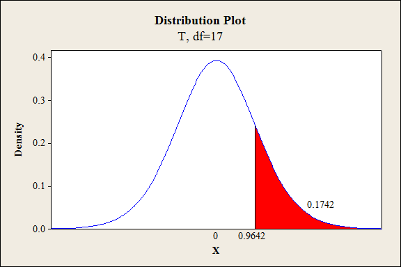
From the output, the P- value is 0.1742.
Thus, the P- value is 0.1742.
Decision criteria based on P-value approach:
If
If
Conclusion:
The P-value is 0.1742 and
Here, P-value is greater than the
That is
By the rejection rule, fail to reject the null hypothesis.
Hence, 1 ppt increase in manganese tends to at most
Therefore, there is no sufficient evidence to conclude that
d.
Test whether there is enough evidence to conclude that
d.
Answer to Problem 2E
There is sufficient evidence to conclude that
Explanation of Solution
Calculation:
From the accompanying MINITAB output, the slope coefficient of Thickness is
Here, the claim is that
The test hypotheses are given below:
Null hypothesis:
That is, 1 mm increase in thickness tends to at least
Alternative hypothesis:
That is, decrease in the true average of tensile strength due to 1 mm increase in thickness will be less than
Test statistic:
The test statistic is,
Where,
From the accompanying MINITAB output, the estimate of error standard deviation of slope coefficient of Thickness is
Test statistic under null hypothesis:
Under the null hypothesis, the test statistic is obtained as follows:
Thus, the test statistic is -2.577.
Degrees of freedom:
The number of plates that are sampled is
The degrees of freedom is,
Thus, the degree of freedom is 17.
Here, level of significance is not given.
So, the prior level of significance
P-value:
Software procedure:
Step by step procedure to obtain the P- value using the MINITAB software:
- Choose Graph > Probability Distribution Plot choose View Probability > OK.
- From Distribution, choose ‘t’ distribution and enter 17 as degrees of freedom.
- Click the Shaded Area tab.
- Choose X-Value and Left Tail for the region of the curve to shade.
- Enter the X-value as -2.577.
- Click OK.
Output obtained from MINITAB is given below:
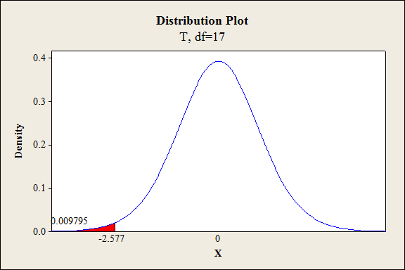
From the output, the P- value is 0.009795.
Thus, the P- value is 0.009795.
Decision criteria based on P-value approach:
If
If
Conclusion:
The P-value is 0.009795 and
Here, P-value is less than the
That is
By the rejection rule, reject the null hypothesis.
Hence, 1 mm increase in thickness tends to at least
Therefore, there is sufficient evidence to conclude that
Want to see more full solutions like this?
Chapter 8 Solutions
Statistics for Engineers and Scientists


- A company found that the daily sales revenue of its flagship product follows a normal distribution with a mean of $4500 and a standard deviation of $450. The company defines a "high-sales day" that is, any day with sales exceeding $4800. please provide a step by step on how to get the answers in excel Q: What percentage of days can the company expect to have "high-sales days" or sales greater than $4800? Q: What is the sales revenue threshold for the bottom 10% of days? (please note that 10% refers to the probability/area under bell curve towards the lower tail of bell curve) Provide answers in the yellow cellsarrow_forwardFind the critical value for a left-tailed test using the F distribution with a 0.025, degrees of freedom in the numerator=12, and degrees of freedom in the denominator = 50. A portion of the table of critical values of the F-distribution is provided. Click the icon to view the partial table of critical values of the F-distribution. What is the critical value? (Round to two decimal places as needed.)arrow_forwardA retail store manager claims that the average daily sales of the store are $1,500. You aim to test whether the actual average daily sales differ significantly from this claimed value. You can provide your answer by inserting a text box and the answer must include: Null hypothesis, Alternative hypothesis, Show answer (output table/summary table), and Conclusion based on the P value. Showing the calculation is a must. If calculation is missing,so please provide a step by step on the answers Numerical answers in the yellow cellsarrow_forward
 Glencoe Algebra 1, Student Edition, 9780079039897...AlgebraISBN:9780079039897Author:CarterPublisher:McGraw Hill
 Big Ideas Math A Bridge To Success Algebra 1: Stu...AlgebraISBN:9781680331141Author:HOUGHTON MIFFLIN HARCOURTPublisher:Houghton Mifflin Harcourt
 Holt Mcdougal Larson Pre-algebra: Student Edition...AlgebraISBN:9780547587776Author:HOLT MCDOUGALPublisher:HOLT MCDOUGAL