
Concept explainers
Videos
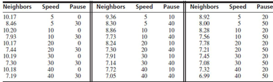
In a simulation of 30 mobile computer networks, the average speed, pause time, and number of neighbor were measured. A “neighbor” is a computer within the transmission
- a. Fit the model with Neighbors as the dependent variable, and independent variables Speed, Pause, Speed,·Pause, Speed2, and Pause2.
- b. Construct a reduced model by dropping any variables whose P-values are large, and test the plausibility of the model with an F test.
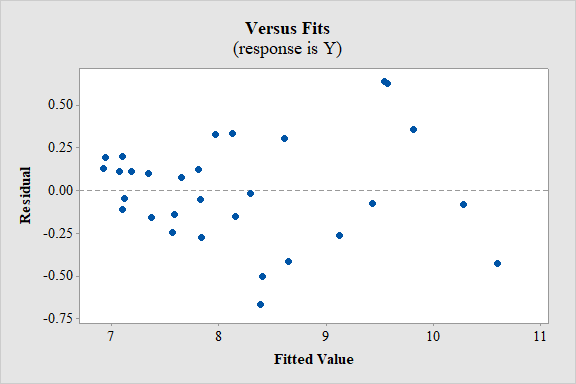
- c. Plot the residuals versus the fitted values for the reduced model. Are there any indications that the model is inappropriate? If so, what are they?
- d. Someone suggests that a model containing Pause and Pause2 as the only dependent variables is adequate. Do you agree? Why or why not?
- e. Using a best subsets software package, find the two models with the highest R2 value for each model size from one to five variables. Compute Cp and adjusted R2 for each model.
- f. Which model is selected by minimum Cp? By adjusted R2? Are they the same?
a.
Construct a multiple linear regression model with neighbor as the dependent variable, speed, pause,
Answer to Problem 5SE
A multiple linear regression model for the given data is:
Explanation of Solution
Calculation:
The data represents the values of the variables number of neighbors, average speed and pause time for a simulation of 30 mobile network computers.
Multiple linear regression model:
A multiple linear regression model is given as
Let
Regression:
Software procedure:
Step by step procedure to obtain regression using MINITAB software is given as,
- Choose Stat > Regression > General Regression.
- In Response, enter the numeric column containing the response data Y.
- In Model, enter the numeric column containing the predictor variables X1, X2, X1*X2, X1*X1 and X2*X2.
- Click OK.
Output obtained from MINITAB is given below:
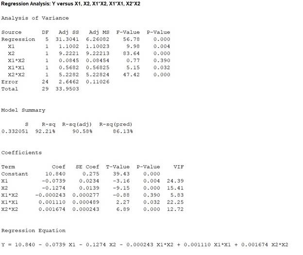
The ‘Coefficient’ column of the regression analysis MINITAB output gives the slopes corresponding to the respective variables stored in the column ‘Term’.
A careful inspection of the output shows that the fitted model is:
Hence, the multiple linear regression model for the given data is:
b.
Construct a reduced model by dropping the variables with large P- values.
Check whether the reduced model is plausible or not.
Answer to Problem 5SE
A multiple linear regression model for the given data is:
Yes, there is enough evidence to conclude that the reduced model is plausible.
Explanation of Solution
Calculation:
From part (a), it can be seen that the ‘P’ column of the regression analysis MINITAB output gives the slopes corresponding to the respective variables stored in the column ‘Term’.
By observing the P- values of the MINITAB output, it is clear that the largest P-value is 0.390 corresponding to the predictor variable
Now, the new regression has to be fitted after dropping the predictor variable
Regression:
Software procedure:
Step by step procedure to obtain regression using MINITAB software is given as,
- Choose Stat > Regression > General Regression.
- In Response, enter the numeric column containing the response data Y.
- In Model, enter the numeric column containing the predictor variables X1, X2, X1*X1 and X2*X2.
- Click OK.
Output obtained from MINITAB is given below:
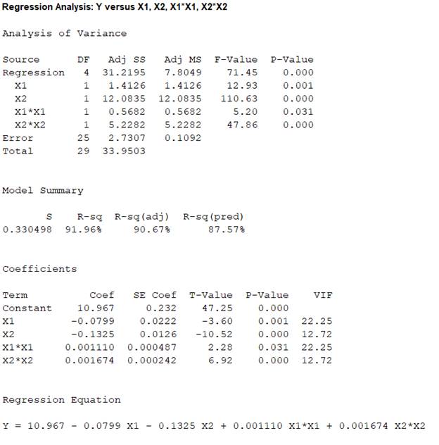
The ‘Coefficient’ column of the regression analysis MINITAB output gives the slopes corresponding to the respective variables stored in the column ‘Term’.
A careful inspection of the output shows that the fitted model is:
Hence, the multiple linear regression model for the given data is:
The full model is,
The reduced model is,
The test hypotheses are given below:
Null hypothesis:
That is, the dropped predictor of the full model is not significant to predict y.
Alternative hypothesis:
That is, the dropped predictor of the full model is significant to predict y.
Test statistic:
Where,
n represents the total number of observations.
p represents the number of predictors on the full model.
k represents the number of predictors on the reduced model.
From the obtained MINITAB outputs, the value of error sum of squares for full model is
The total number of observations is
Number of predictors on the full model is
Degrees of freedom of F-statistic for reduced model:
In a reduced multiple linear regression analysis, the F-statistic is
In the ratio, the numerator is obtained by dividing the quantity
Thus, the degrees of freedom for the F-statistic in a reduced multiple regression analysis are
Hence, the numerator degrees of freedom is
Test statistic under null hypothesis:
Under the null hypothesis, the test statistic is obtained as follows:
Thus, the test statistic is
Since, the level of significance is not specified. The prior level of significance
P-value:
Software procedure:
- Choose Graph > Probability Distribution Plot choose View Probability > OK.
- From Distribution, choose F, enter 1 in numerator df and 24 in denominator df.
- Click the Shaded Area tab.
- Choose X-Value and Right Tail for the region of the curve to shade.
- Enter the X-value as 0.76638.
- Click OK.
Output obtained from MINITAB is given below:
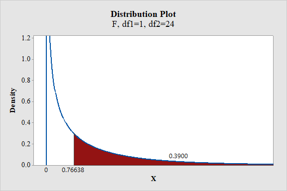
From the output, the P- value is 0.39.
Thus, the P- value is 0.39.
Decision criteria based on P-value approach:
If
If
Conclusion:
The P-value is 0.39 and
Here, P-value is greater than the
That is
By the rejection rule, fail to reject the null hypothesis.
Hence, there is sufficient evidence to conclude that the dropped predictor variable is not significant to predict the response variable y.
Thus, the reduced model is useful than the full model to predict the response variable y.
c.
Plot the residuals versus fitted line plot for the reduced model.
Check whether the model is appropriate.
Answer to Problem 5SE
Residual plot:
Yes, the model seems to be appropriate.
Explanation of Solution
Calculation:
Residual plot:
Software procedure:
Step by step procedure to obtain regression using MINITAB software is given as,
- Choose Stat > Regression > General Regression.
- In Response, enter the numeric column containing the response data Y.
- In Model, enter the numeric column containing the predictor variables X1, X2, X1*X1 and X2*X2.
- In Graphs, Under Residuals for plots, select Regular.
- Under Residual plots select box Residuals versus fits.
- Click OK.
Conditions for the appropriateness of regression model using the residual plot:
- The plot of the residuals vs. fitted values should fall roughly in a horizontal band contended and symmetric about x-axis. That is, the residuals of the data should not represent any bend.
- The plot of residuals should not contain any outliers.
- The residuals have to be scattered randomly around “0” with constant variability among for all the residuals. That is, the spread should be consistent.
Interpretation:
In residual plot there is high bend or pattern, which can violate the straight line condition and there is change in the spread of the residuals from one part to another part of the plot.
However, it is difficult to determine about the violation of the assumptions without the data.
Thus, the model seems to be appropriate.
d.
Check whether the model with only two dependent variables
Answer to Problem 5SE
No, the model with only two dependent variables
Explanation of Solution
Calculation:
Regression:
Software procedure:
Step by step procedure to obtain regression using MINITAB software is given as,
- Choose Stat > Regression > General Regression.
- In Response, enter the numeric column containing the response data Y.
- In Model, enter the numeric column containing the predictor variables X2 and X2*X2.
- Click OK.
Output obtained from MINITAB is given below:
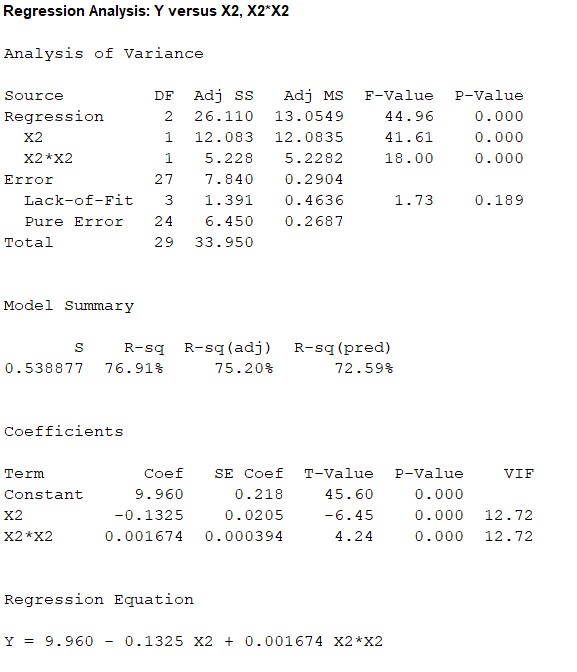
The ‘Coefficient’ column of the regression analysis MINITAB output gives the slopes corresponding to the respective variables stored in the column ‘Term’.
A careful inspection of the output shows that the fitted model is:
Hence, the multiple linear regression model for the given data is:
The full model is,
The reduced model is,
The test hypotheses are given below:
Null hypothesis:
That is, the dropped predictors of the full model are not significant to predict y.
Alternative hypothesis:
That is, at least one of the dropped predictors of the full model are significant to predict y.
Test statistic:
Where,
n represents the total number of observations.
p represents the number of predictors on the full model.
k represents the number of predictors on the reduced model.
From the obtained MINITAB outputs, the value of error sum of squares for full model is
The total number of observations is
Number of predictors on the full model is
Degrees of freedom of F-statistic for reduced model:
In a reduced multiple linear regression analysis, the F-statistic is
In the ratio, the numerator is obtained by dividing the quantity
Thus, the degrees of freedom for the F-statistic in a reduced multiple regression analysis are
Hence, the numerator degrees of freedom is
Test statistic under null hypothesis:
Under the null hypothesis, the test statistic is obtained as follows:
Thus, the test statistic is
Since, the level of significance is not specified. The prior level of significance
P-value:
Software procedure:
- Choose Graph > Probability Distribution Plot choose View Probability > OK.
- From Distribution, choose F, enter 3 in numerator df and 24 in denominator df.
- Click the Shaded Area tab.
- Choose X-Value and Right Tail for the region of the curve to shade.
- Enter the X-value as 15.702.
- Click OK.
Output obtained from MINITAB is given below:
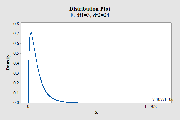
From the output, the P- value is
Thus, the P- value is
Decision criteria based on P-value approach:
If
If
Conclusion:
The P-value is
Here, P-value is less than the
That is
By the rejection rule, reject the null hypothesis.
Hence, there is sufficient evidence to conclude that at least one of the dropped predictors of the full model are significant to predict y.
Thus, the model with only two dependent variables
e.
Find the two models with the highest
Obtain the values of mallows
Answer to Problem 5SE
The two models with the highest
First model with
The values of M Mallows’
| Predictor variables | Mallows’ | Adjusted |
| 92.5 | 60.1 | |
| 97 | 58.6 | |
| 47.1 | 75.2 | |
| 53.3 | 73 | |
| 7.9 | 89.2 | |
| 15.5 | 86.4 | |
| 4.8 | 90.7 | |
| 9.2 | 89 | |
| 6 | 90.6 |
Explanation of Solution
Calculation:
Coefficient of multiple determination
The coefficient of multiple determination,
The subset with larger
Regression:
Software procedure:
Step by step procedure to obtain regression using MINITAB software is given as,
- Choose Stat > Regression > Regression> Best subsets.
- In Response, enter the numeric column containing the response data Y.
- In Model, enter the numeric column containing the predictor variables X1, X2, X1*X2, X1*X1 and X2*X2.
- Click OK.
Output obtained from MINITAB is given below:
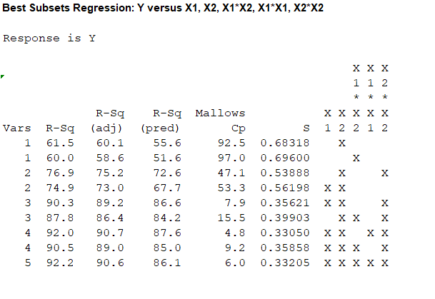
For the one predictor case, the highest value of
For the two predictor case, the highest value of
For the three predictor case, the highest value of
For the four predictor case, the highest value of
For the five predictor case, the value of
The value of
Thus, depending upon the factors affecting the analysis it would be most preferable to use the regression equation corresponding to the predictors
The second highest value of
That is, 90.6 and 90.3 are not much distinct.
Therefore, the model with
Thus, the two best models are:
First model with
From the accompanying MINITAB output, the values of Mallows’
| Predictor variables | Mallows’ | Adjusted |
| 92.5 | 60.1 | |
| 97 | 58.6 | |
| 47.1 | 75.2 | |
| 53.3 | 73 | |
| 7.9 | 89.2 | |
| 15.5 | 86.4 | |
| 4.8 | 90.7 | |
| 9.2 | 89 | |
| 6 | 90.6 |
f.
Select the variables for the model, using the Mallows’
Check whether both the models are same.
Answer to Problem 5SE
The variables for the model using the Mallows’
The variables for the model using the adjusted-
Yes, both the models are same.
Explanation of Solution
Mallows’
An important utility of the Mallows’
Mallows’
The predictor with the lowest value of
From part (e), the values of Mallows’
| Predictor variables | Mallows’ | Adjusted |
| 92.5 | 60.1 | |
| 97 | 58.6 | |
| 47.1 | 75.2 | |
| 53.3 | 73 | |
| 7.9 | 89.2 | |
| 15.5 | 86.4 | |
| 4.8 | 90.7 | |
| 9.2 | 89 | |
| 6 | 90.6 |
For the one predictor case, the lowest value of
For the two predictor case, the lowest value of
For the three predictor case, the lowest value of
For the four predictor case, the lowest value of
For the five predictor case, the value of
The value of
Thus, depending upon the factors affecting the analysis it would be most preferable to use the regression equation corresponding to the predictors
Hence, the variables for the model using the Mallows’
Adjusted
An important utility of the adjusted coefficient of multiple determination or
The adjusted coefficient of multiple determination,
For the one predictor case, the highest value of
For the two predictor case, the highest value of
For the three predictor case, the highest value of
For the four predictor case, the highest value of
For the five predictor case, the value of
The value of adjusted
Thus, provided other factors do not affect the analysis it could be most preferable to use the regression equation corresponding to the predictors,
Hence, the variables for the model using the adjusted-
Both Mallows’
Want to see more full solutions like this?
Chapter 8 Solutions
Statistics for Engineers and Scientists
Additional Math Textbook Solutions
Math in Our World
Elementary Statistics ( 3rd International Edition ) Isbn:9781260092561
APPLIED STAT.IN BUS.+ECONOMICS
Introductory Statistics
Elementary Statistics: Picturing the World (7th Edition)
Mathematics for the Trades: A Guided Approach (11th Edition) (What's New in Trade Math)


- Harvard University California Institute of Technology Massachusetts Institute of Technology Stanford University Princeton University University of Cambridge University of Oxford University of California, Berkeley Imperial College London Yale University University of California, Los Angeles University of Chicago Johns Hopkins University Cornell University ETH Zurich University of Michigan University of Toronto Columbia University University of Pennsylvania Carnegie Mellon University University of Hong Kong University College London University of Washington Duke University Northwestern University University of Tokyo Georgia Institute of Technology Pohang University of Science and Technology University of California, Santa Barbara University of British Columbia University of North Carolina at Chapel Hill University of California, San Diego University of Illinois at Urbana-Champaign National University of Singapore McGill…arrow_forwardName Harvard University California Institute of Technology Massachusetts Institute of Technology Stanford University Princeton University University of Cambridge University of Oxford University of California, Berkeley Imperial College London Yale University University of California, Los Angeles University of Chicago Johns Hopkins University Cornell University ETH Zurich University of Michigan University of Toronto Columbia University University of Pennsylvania Carnegie Mellon University University of Hong Kong University College London University of Washington Duke University Northwestern University University of Tokyo Georgia Institute of Technology Pohang University of Science and Technology University of California, Santa Barbara University of British Columbia University of North Carolina at Chapel Hill University of California, San Diego University of Illinois at Urbana-Champaign National University of Singapore…arrow_forwardA company found that the daily sales revenue of its flagship product follows a normal distribution with a mean of $4500 and a standard deviation of $450. The company defines a "high-sales day" that is, any day with sales exceeding $4800. please provide a step by step on how to get the answers in excel Q: What percentage of days can the company expect to have "high-sales days" or sales greater than $4800? Q: What is the sales revenue threshold for the bottom 10% of days? (please note that 10% refers to the probability/area under bell curve towards the lower tail of bell curve) Provide answers in the yellow cellsarrow_forward
- Find the critical value for a left-tailed test using the F distribution with a 0.025, degrees of freedom in the numerator=12, and degrees of freedom in the denominator = 50. A portion of the table of critical values of the F-distribution is provided. Click the icon to view the partial table of critical values of the F-distribution. What is the critical value? (Round to two decimal places as needed.)arrow_forwardA retail store manager claims that the average daily sales of the store are $1,500. You aim to test whether the actual average daily sales differ significantly from this claimed value. You can provide your answer by inserting a text box and the answer must include: Null hypothesis, Alternative hypothesis, Show answer (output table/summary table), and Conclusion based on the P value. Showing the calculation is a must. If calculation is missing,so please provide a step by step on the answers Numerical answers in the yellow cellsarrow_forwardShow all workarrow_forward
 Functions and Change: A Modeling Approach to Coll...AlgebraISBN:9781337111348Author:Bruce Crauder, Benny Evans, Alan NoellPublisher:Cengage Learning
 Holt Mcdougal Larson Pre-algebra: Student Edition...AlgebraISBN:9780547587776Author:HOLT MCDOUGALPublisher:HOLT MCDOUGAL
 Big Ideas Math A Bridge To Success Algebra 1: Stu...AlgebraISBN:9781680331141Author:HOUGHTON MIFFLIN HARCOURTPublisher:Houghton Mifflin Harcourt