
Introduction To Statistics And Data Analysis
6th Edition
ISBN: 9781337793612
Author: PECK, Roxy.
Publisher: Cengage Learning,
expand_more
expand_more
format_list_bulleted
Concept explainers
Videos
Textbook Question
Chapter 3.3, Problem 31E
Use the commute time data given in the previous exercise to complete the following:
- a. Calculate the cumulative relative frequencies, and construct a cumulative relative frequency plot.
- b. Use the cumulative relative frequency plot constructed in Part (a) to answer the following questions.
- i. Approximately what proportion of commute times were less than 50 minutes?
- ii. Approximately what proportion of commute times were greater than 22 minutes?
- iii. What is the approximate commute time value that separates the shortest 50% of commute times from the longest 50%?
3.30 U.S. Census data for San Luis Obispo County, California, were used to construct the following relative frequency distribution for commute time (in minutes) of working adults in 2015 (datausa.io/profile/geo/san-luis-bispo-paso-robles-ca-metro-area/#housing, retrieved February 18, 2018) and so are only approximate):
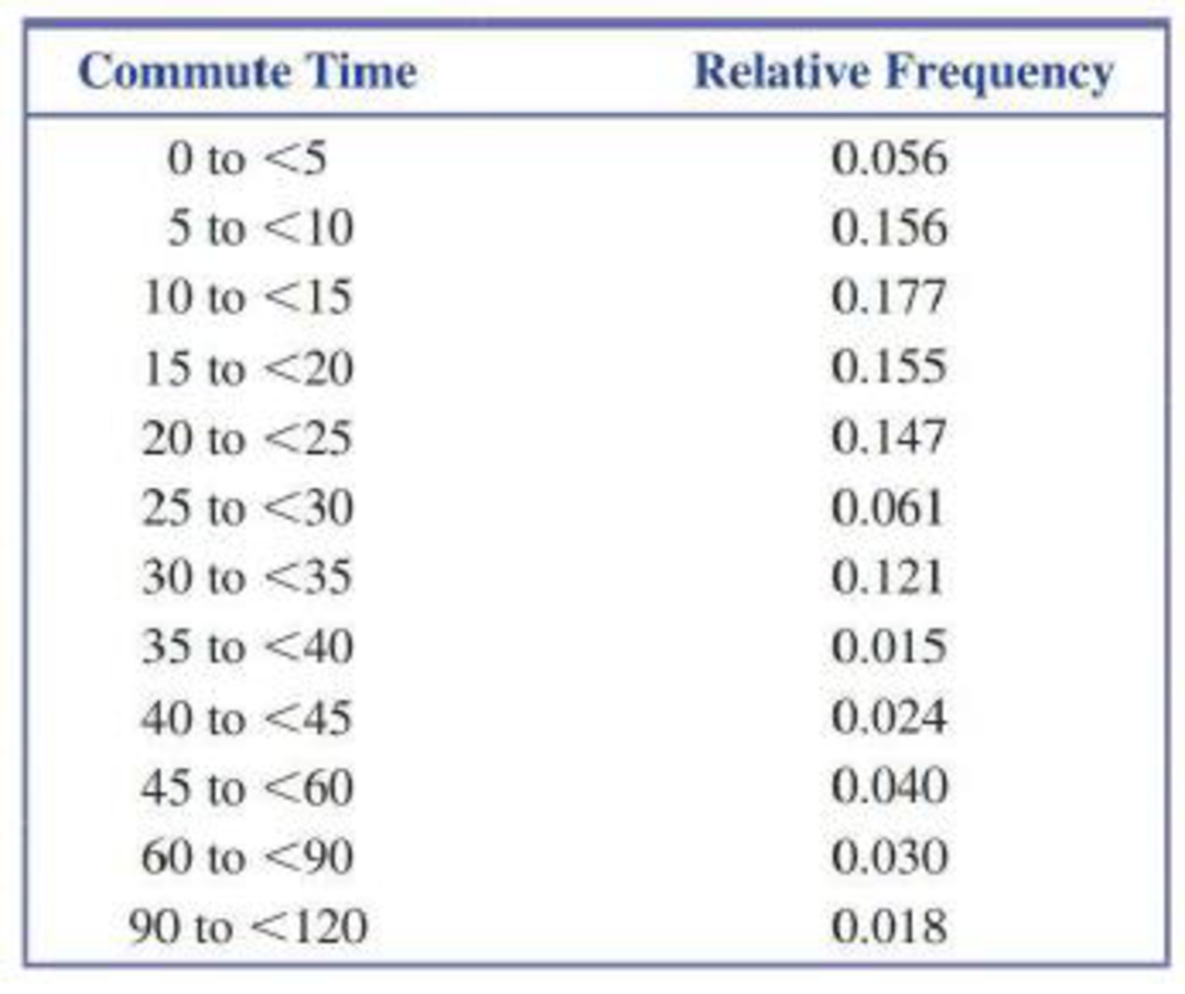
- a. Notice that not all intervals in the frequency distribution are equal in width. Why do you think that unequal width intervals were used?
- b. Construct a table that adds a density column to the given relative frequency distribution. (Hint: See Example 3.17.)
- c. Use the densities computed in Part (b) to construct a histogram for this data set. (The web site referenced earlier actually displays an incorrectly drawn histogram based on relative frequencies rather than densities!) Write a few sentences commenting on the important features of the histogram.
Expert Solution & Answer

Trending nowThis is a popular solution!

Students have asked these similar questions
Q.2.4 There are twelve (12) teams participating in a pub quiz. What is the probability of correctly predicting the top three teams at the end of the competition, in the correct order? Give your final answer as a fraction in its simplest form.
The table below indicates the number of years of experience of a sample of employees who work on a particular production line and the corresponding number of units of a good that each employee produced last month.
Years of Experience (x)
Number of Goods (y)
11
63
5
57
1
48
4
54
5
45
3
51
Q.1.1 By completing the table below and then applying the relevant formulae, determine the line of best fit for this bivariate data set.
Do NOT change the units for the variables.
X
y
X2
xy
Ex=
Ey=
EX2
EXY=
Q.1.2 Estimate the number of units of the good that would have been produced last month by an employee with 8 years of experience.
Q.1.3 Using your calculator, determine the coefficient of correlation for the data set.
Interpret your answer.
Q.1.4 Compute the coefficient of determination for the data set.
Interpret your answer.
Can you answer this question for me
Chapter 3 Solutions
Introduction To Statistics And Data Analysis
Ch. 3.1 - Each person in a nationally representative sample...Ch. 3.1 - The graphical display on the next page is similar...Ch. 3.1 - The survey referenced in the previous exercise was...Ch. 3.1 - The National Confectioners Association asked 1006...Ch. 3.1 - College student attitudes about e-books were...Ch. 3.1 - The Center for Science in the Public Interest...Ch. 3.1 - Using the data given in the previous exercise,...Ch. 3.1 - The article Housework around the World (USA TODAY,...Ch. 3.1 - The authors of the report Findings from the 2009...Ch. 3.1 - The survey on student attitude toward e-books...
Ch. 3.1 - During 2017, Gallup conducted a survey of adult...Ch. 3.1 - An article about college loans (New Rules Would...Ch. 3.1 - The report Findings From the 2014 College Senior...Ch. 3.2 - The National Center for Health Statistics provided...Ch. 3.2 - The paper State-Level Cancer Mortality...Ch. 3.2 - The accompanying data on seat belt use for each of...Ch. 3.2 - The previous exercise gave data on seat belt use...Ch. 3.2 - The U.S. Department of Health and Human Services...Ch. 3.2 - The article Economy Low, Generosity High (USA...Ch. 3.2 - The U.S. gasoline tax per gallon data for each of...Ch. 3.2 - A report from Texas Transportation Institute...Ch. 3.2 - The percentage of teens not in school or working...Ch. 3.3 - The data in the accompanying table are from the...Ch. 3.3 - The accompanying data on annual maximum wind speed...Ch. 3.3 - The accompanying relative frequency table is based...Ch. 3.3 - The data in the accompanying table represents the...Ch. 3.3 - Construct a histogram for the data in the previous...Ch. 3.3 - The following two relative frequency distributions...Ch. 3.3 - U.S. Census data for San Luis Obispo County,...Ch. 3.3 - Use the commute time data given in the previous...Ch. 3.3 - The report Trends in College Pricing 2012...Ch. 3.3 - An exam is given to students in an introductory...Ch. 3.3 - The accompanying frequency distribution summarizes...Ch. 3.3 - Example 3.19 used annual rainfall data for...Ch. 3.3 - Use the relative frequency distribution...Ch. 3.3 - Prob. 37ECh. 3.3 - Use the cumulative relative frequencies given in...Ch. 3.3 - Using the five class intervals 100 to 120, 120 to...Ch. 3.4 - The accompanying table gives data from a survey of...Ch. 3.4 - Consumer Reports Health (consumerreports.org) gave...Ch. 3.4 - Consumer Reports rated 29 fitness trackers (such...Ch. 3.4 - Consumer Reports (consumerreports.org) rated 37...Ch. 3.4 - The Solid Waste Management section of the...Ch. 3.4 - The report Daily Cigarette Use: Indicators on...Ch. 3.4 - The accompanying time series plot of movie box...Ch. 3.5 - The accompanying comparative bar chart is similar...Ch. 3.5 - The figure at the top left of the next page is...Ch. 3.5 - The figure at the top right of the next page is...Ch. 3.5 - The two graphical displays below are similar to...Ch. 3.5 - The following graphical display is similar to one...Ch. 3.5 - Explain why the following graphical display...Ch. 3 - Each year, The Princeton Review conducts surveys...Ch. 3 - Prob. 55CRCh. 3 - Prob. 56CRCh. 3 - Prob. 57CRCh. 3 - Prob. 58CRCh. 3 - Does the size of a transplanted organ matter? A...Ch. 3 - Prob. 60CRCh. 3 - The article Tobacco and Alcohol Use in G-Rated...Ch. 3 - Prob. 62CRCh. 3 - Prob. 63CRCh. 3 - Many nutritional experts have expressed concern...Ch. 3 - Americium 241 (241Am) is a radioactive material...Ch. 3 - Does eating broccoli reduce the risk of prostate...Ch. 3 - An article that appeared in USA TODAY (August 11,...Ch. 3 - Sometimes samples are composed entirely of...Ch. 3 - Prob. 4CRECh. 3 - More than half of Californias doctors say they are...Ch. 3 - Based on observing more than 400 drivers in the...Ch. 3 - An article from the Associated Press (May 14,...Ch. 3 - Prob. 8CRECh. 3 - Prob. 9CRECh. 3 - Prob. 10CRECh. 3 - The article Determination of Most Representative...Ch. 3 - The paper Lessons from Pacemaker Implantations...Ch. 3 - How does the speed of a runner vary over the...Ch. 3 - Prob. 14CRECh. 3 - One factor in the development of tennis elbow, a...Ch. 3 - An article that appeared in USA TODAY (September...
Additional Math Textbook Solutions
Find more solutions based on key concepts
Complete each statement with the correct term from the column on the right. Some of the choices may not be used...
Intermediate Algebra (13th Edition)
Provide an example of a qualitative variable and an example of a quantitative variable.
Elementary Statistics ( 3rd International Edition ) Isbn:9781260092561
True or False The quotient of two polynomial expressions is a rational expression, (p. A35)
Precalculus
1. How much money is Joe earning when he’s 30?
Pathways To Math Literacy (looseleaf)
(a) Make a stem-and-leaf plot for these 24 observations on the number of customers who used a down-town CitiBan...
APPLIED STAT.IN BUS.+ECONOMICS
Evaluate the integrals in Exercises 1–46.
1.
University Calculus: Early Transcendentals (4th Edition)
Knowledge Booster


Learn more about
Need a deep-dive on the concept behind this application? Look no further. Learn more about this topic, statistics and related others by exploring similar questions and additional content below.Similar questions
- Techniques QUAT6221 2025 PT B... TM Tabudi Maphoru Activities Assessments Class Progress lIE Library • Help v The table below shows the prices (R) and quantities (kg) of rice, meat and potatoes items bought during 2013 and 2014: 2013 2014 P1Qo PoQo Q1Po P1Q1 Price Ро Quantity Qo Price P1 Quantity Q1 Rice 7 80 6 70 480 560 490 420 Meat 30 50 35 60 1 750 1 500 1 800 2 100 Potatoes 3 100 3 100 300 300 300 300 TOTAL 40 230 44 230 2 530 2 360 2 590 2 820 Instructions: 1 Corall dawn to tha bottom of thir ceraan urina se se tha haca nariad in archerca antarand cubmit Q Search ENG US 口X 2025/05arrow_forwardThe table below indicates the number of years of experience of a sample of employees who work on a particular production line and the corresponding number of units of a good that each employee produced last month. Years of Experience (x) Number of Goods (y) 11 63 5 57 1 48 4 54 45 3 51 Q.1.1 By completing the table below and then applying the relevant formulae, determine the line of best fit for this bivariate data set. Do NOT change the units for the variables. X y X2 xy Ex= Ey= EX2 EXY= Q.1.2 Estimate the number of units of the good that would have been produced last month by an employee with 8 years of experience. Q.1.3 Using your calculator, determine the coefficient of correlation for the data set. Interpret your answer. Q.1.4 Compute the coefficient of determination for the data set. Interpret your answer.arrow_forwardQ.3.2 A sample of consumers was asked to name their favourite fruit. The results regarding the popularity of the different fruits are given in the following table. Type of Fruit Number of Consumers Banana 25 Apple 20 Orange 5 TOTAL 50 Draw a bar chart to graphically illustrate the results given in the table.arrow_forward
- Q.2.3 The probability that a randomly selected employee of Company Z is female is 0.75. The probability that an employee of the same company works in the Production department, given that the employee is female, is 0.25. What is the probability that a randomly selected employee of the company will be female and will work in the Production department? Q.2.4 There are twelve (12) teams participating in a pub quiz. What is the probability of correctly predicting the top three teams at the end of the competition, in the correct order? Give your final answer as a fraction in its simplest form.arrow_forwardQ.2.1 A bag contains 13 red and 9 green marbles. You are asked to select two (2) marbles from the bag. The first marble selected will not be placed back into the bag. Q.2.1.1 Construct a probability tree to indicate the various possible outcomes and their probabilities (as fractions). Q.2.1.2 What is the probability that the two selected marbles will be the same colour? Q.2.2 The following contingency table gives the results of a sample survey of South African male and female respondents with regard to their preferred brand of sports watch: PREFERRED BRAND OF SPORTS WATCH Samsung Apple Garmin TOTAL No. of Females 30 100 40 170 No. of Males 75 125 80 280 TOTAL 105 225 120 450 Q.2.2.1 What is the probability of randomly selecting a respondent from the sample who prefers Garmin? Q.2.2.2 What is the probability of randomly selecting a respondent from the sample who is not female? Q.2.2.3 What is the probability of randomly…arrow_forwardTest the claim that a student's pulse rate is different when taking a quiz than attending a regular class. The mean pulse rate difference is 2.7 with 10 students. Use a significance level of 0.005. Pulse rate difference(Quiz - Lecture) 2 -1 5 -8 1 20 15 -4 9 -12arrow_forward
- The following ordered data list shows the data speeds for cell phones used by a telephone company at an airport: A. Calculate the Measures of Central Tendency from the ungrouped data list. B. Group the data in an appropriate frequency table. C. Calculate the Measures of Central Tendency using the table in point B. D. Are there differences in the measurements obtained in A and C? Why (give at least one justified reason)? I leave the answers to A and B to resolve the remaining two. 0.8 1.4 1.8 1.9 3.2 3.6 4.5 4.5 4.6 6.2 6.5 7.7 7.9 9.9 10.2 10.3 10.9 11.1 11.1 11.6 11.8 12.0 13.1 13.5 13.7 14.1 14.2 14.7 15.0 15.1 15.5 15.8 16.0 17.5 18.2 20.2 21.1 21.5 22.2 22.4 23.1 24.5 25.7 28.5 34.6 38.5 43.0 55.6 71.3 77.8 A. Measures of Central Tendency We are to calculate: Mean, Median, Mode The data (already ordered) is: 0.8, 1.4, 1.8, 1.9, 3.2, 3.6, 4.5, 4.5, 4.6, 6.2, 6.5, 7.7, 7.9, 9.9, 10.2, 10.3, 10.9, 11.1, 11.1, 11.6, 11.8, 12.0, 13.1, 13.5, 13.7, 14.1, 14.2, 14.7, 15.0, 15.1, 15.5,…arrow_forwardPEER REPLY 1: Choose a classmate's Main Post. 1. Indicate a range of values for the independent variable (x) that is reasonable based on the data provided. 2. Explain what the predicted range of dependent values should be based on the range of independent values.arrow_forwardIn a company with 80 employees, 60 earn $10.00 per hour and 20 earn $13.00 per hour. Is this average hourly wage considered representative?arrow_forward
- The following is a list of questions answered correctly on an exam. Calculate the Measures of Central Tendency from the ungrouped data list. NUMBER OF QUESTIONS ANSWERED CORRECTLY ON AN APTITUDE EXAM 112 72 69 97 107 73 92 76 86 73 126 128 118 127 124 82 104 132 134 83 92 108 96 100 92 115 76 91 102 81 95 141 81 80 106 84 119 113 98 75 68 98 115 106 95 100 85 94 106 119arrow_forwardThe following ordered data list shows the data speeds for cell phones used by a telephone company at an airport: A. Calculate the Measures of Central Tendency using the table in point B. B. Are there differences in the measurements obtained in A and C? Why (give at least one justified reason)? 0.8 1.4 1.8 1.9 3.2 3.6 4.5 4.5 4.6 6.2 6.5 7.7 7.9 9.9 10.2 10.3 10.9 11.1 11.1 11.6 11.8 12.0 13.1 13.5 13.7 14.1 14.2 14.7 15.0 15.1 15.5 15.8 16.0 17.5 18.2 20.2 21.1 21.5 22.2 22.4 23.1 24.5 25.7 28.5 34.6 38.5 43.0 55.6 71.3 77.8arrow_forwardIn a company with 80 employees, 60 earn $10.00 per hour and 20 earn $13.00 per hour. a) Determine the average hourly wage. b) In part a), is the same answer obtained if the 60 employees have an average wage of $10.00 per hour? Prove your answer.arrow_forward
arrow_back_ios
SEE MORE QUESTIONS
arrow_forward_ios
Recommended textbooks for you
 Holt Mcdougal Larson Pre-algebra: Student Edition...AlgebraISBN:9780547587776Author:HOLT MCDOUGALPublisher:HOLT MCDOUGAL
 College Algebra (MindTap Course List)AlgebraISBN:9781305652231Author:R. David Gustafson, Jeff HughesPublisher:Cengage Learning
 Algebra: Structure And Method, Book 1AlgebraISBN:9780395977224Author:Richard G. Brown, Mary P. Dolciani, Robert H. Sorgenfrey, William L. ColePublisher:McDougal Littell
 Functions and Change: A Modeling Approach to Coll...AlgebraISBN:9781337111348Author:Bruce Crauder, Benny Evans, Alan NoellPublisher:Cengage Learning
 Big Ideas Math A Bridge To Success Algebra 1: Stu...AlgebraISBN:9781680331141Author:HOUGHTON MIFFLIN HARCOURTPublisher:Houghton Mifflin Harcourt
 Glencoe Algebra 1, Student Edition, 9780079039897...AlgebraISBN:9780079039897Author:CarterPublisher:McGraw Hill
Holt Mcdougal Larson Pre-algebra: Student Edition...
Algebra
ISBN:9780547587776
Author:HOLT MCDOUGAL
Publisher:HOLT MCDOUGAL
College Algebra (MindTap Course List)
Algebra
ISBN:9781305652231
Author:R. David Gustafson, Jeff Hughes
Publisher:Cengage Learning
Algebra: Structure And Method, Book 1
Algebra
ISBN:9780395977224
Author:Richard G. Brown, Mary P. Dolciani, Robert H. Sorgenfrey, William L. Cole
Publisher:McDougal Littell
Functions and Change: A Modeling Approach to Coll...
Algebra
ISBN:9781337111348
Author:Bruce Crauder, Benny Evans, Alan Noell
Publisher:Cengage Learning
Big Ideas Math A Bridge To Success Algebra 1: Stu...
Algebra
ISBN:9781680331141
Author:HOUGHTON MIFFLIN HARCOURT
Publisher:Houghton Mifflin Harcourt
Glencoe Algebra 1, Student Edition, 9780079039897...
Algebra
ISBN:9780079039897
Author:Carter
Publisher:McGraw Hill
The Shape of Data: Distributions: Crash Course Statistics #7; Author: CrashCourse;https://www.youtube.com/watch?v=bPFNxD3Yg6U;License: Standard YouTube License, CC-BY
Shape, Center, and Spread - Module 20.2 (Part 1); Author: Mrmathblog;https://www.youtube.com/watch?v=COaid7O_Gag;License: Standard YouTube License, CC-BY
Shape, Center and Spread; Author: Emily Murdock;https://www.youtube.com/watch?v=_YyW0DSCzpM;License: Standard Youtube License