
Videos
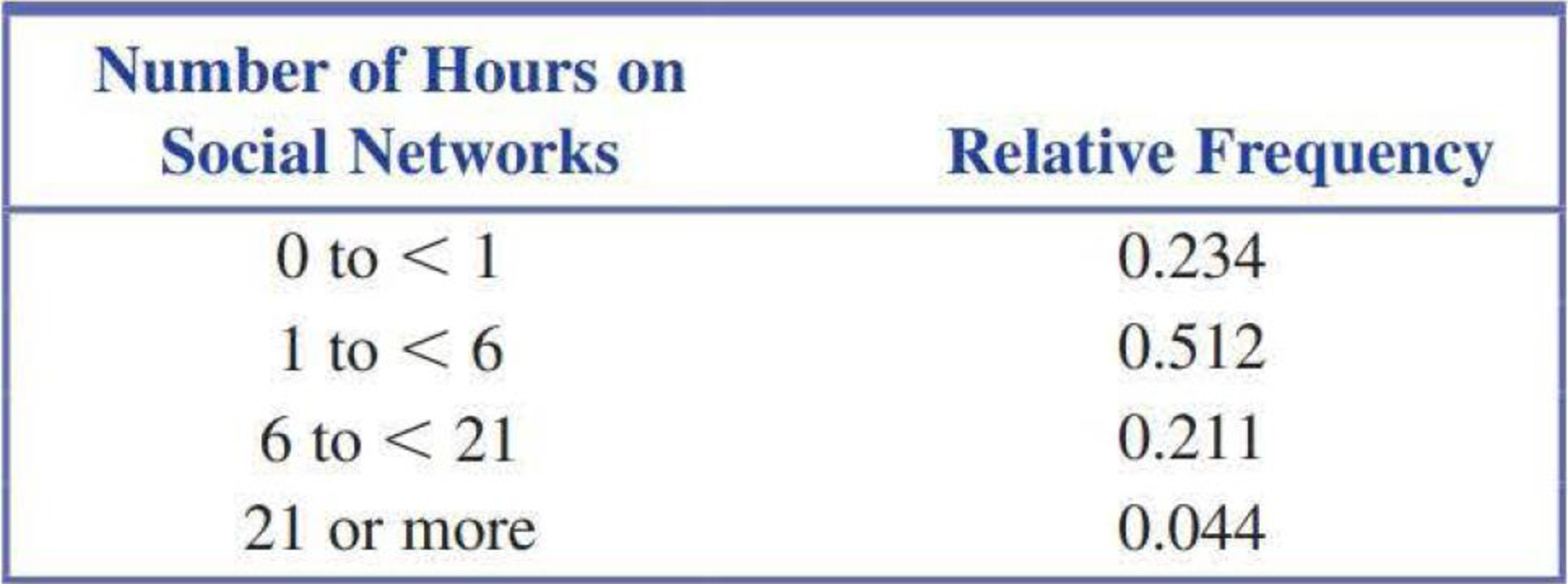
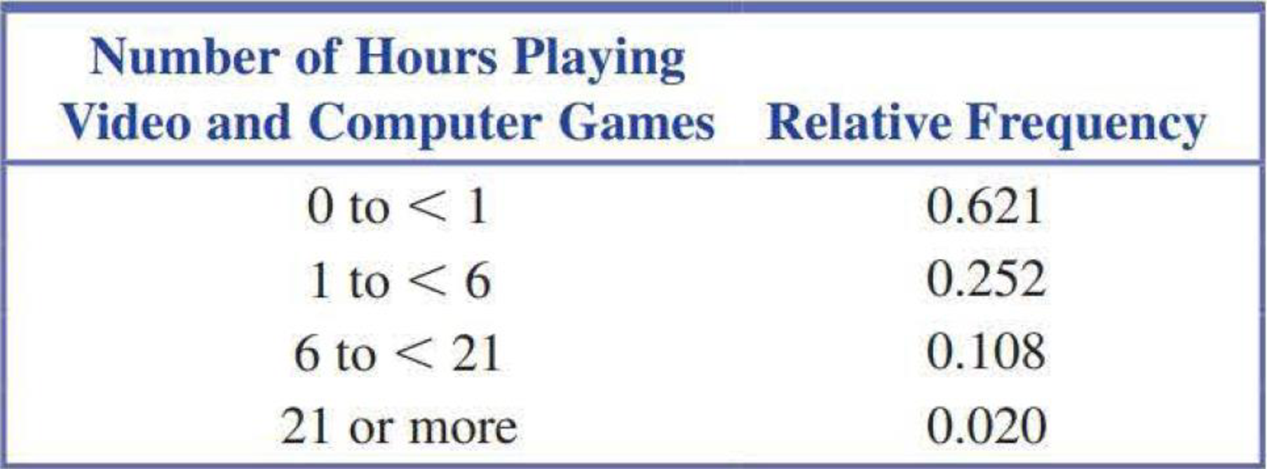
The following two relative frequency distributions are based on data that appeared in The Chronicle of Higher Education (August 23, 2013). The data are from a survey of students at four-year colleges. One relative frequency distribution is for the number of hours spent online at social network sites in a typical week. The second relative frequency distribution is for the number of hours spent playing video and computer games in a typical week.
- a. Construct a histogram for the social media data. For purposes of constructing the histogram, assume that none of the students in the sample spent more than 40 hours on social media in a typical week and that the last interval can be regarded as 21 to <40. Be sure to use the density scale when constructing the histogram. (Hint: See Example 3.17.)
- b. Construct a histogram for the video and computer game data. Use the same scale that you used for the histogram in Part (a) so that it will be easy to compare the two histograms.
- c. Comment on the similarities and differences in the histograms from Parts (a) and (b).
a.
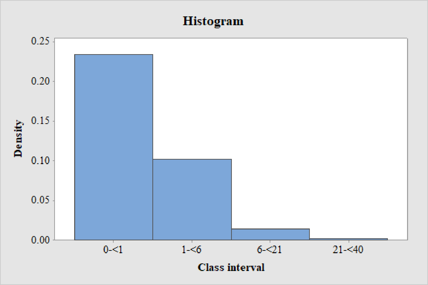
Draw the histogram for the social media data.
Answer to Problem 29E
Output using MINITAB is given below.
Explanation of Solution
Calculation:
The data represents the relative frequency distribution for the number of hours spent online at social network by students at four year colleges. The maximum value is given as 40.
For the continuous data with unequal class width, the vertical scale of the histogram must be density scale. The rectangle heights are the densities of the intervals.
Here, the class intervals do not have equal length. Hence, the histogram with the relative frequencies is not appropriate.
Therefore, the density of the data has to be used to draw a histogram.
The general formula for the rectangle height or density is,
Densities of class intervals:
Substitute the relative frequency of the class interval 0-<1 as “0.234”.
Substitute class width as,
Therefore, the density of the class intervals 0-<1 is,
Similarly, densities for the remaining class intervals are obtained below:
| Class interval | Relative frequency | Class width | Density |
| 0-<1 | 0.234 | ||
| 1-<6 | 0.512 | ||
| 6-<21 | 0.211 | ||
| 21-<40 | 0.044 |
Histogram:
Software procedure:
Step by step procedure to draw the histogram using MINITAB software.
- Select Graph > Bar chart.
- In Bars represent select values from a table.
- In one column of values select Simple.
- Enter density in Graph variables.
- Enter Class interval in categorical variable.
- In gap between clusters enter 0.
- Select OK.
Observation:
From the histogram, it is observed that the distribution of number of hours spent online at social network is positively skewed with single mode.
b.
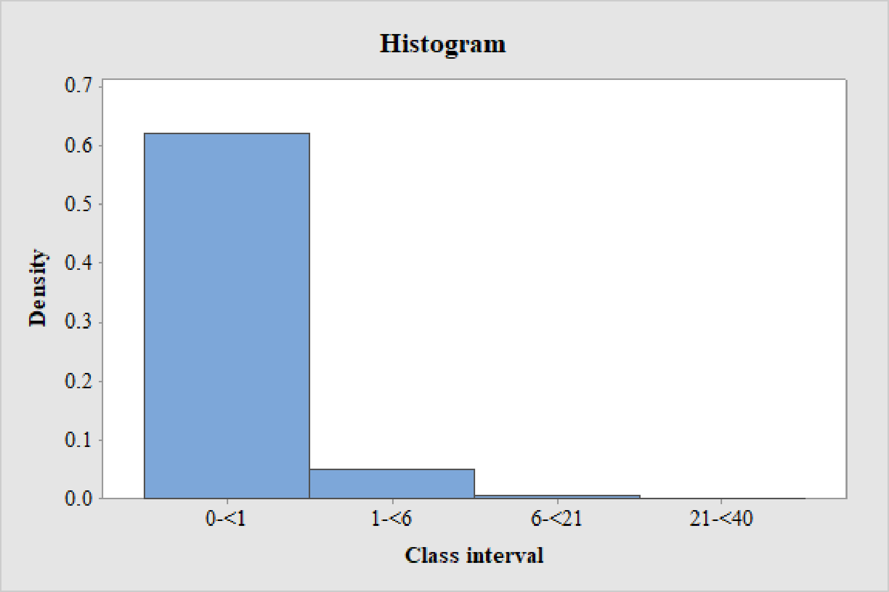
Draw the histogram for the video and computer games data.
Answer to Problem 29E
Output using MINITAB is given below.
Explanation of Solution
Calculation:
The data represents the relative frequency distribution for the number of hours spent playing video and computer games in a typical week by students at four year colleges.
For the continuous data with unequal class width, the vertical scale of the histogram must be density scale. The rectangle heights are the densities of the intervals.
Here, the class intervals do not have equal length. Hence, the histogram with the relative frequencies is not appropriate.
Therefore, the density of the angry intensity tantrum has to be used to draw a histogram.
The general formula for the rectangle height or density is,
Densities of class intervals:
Substitute the relative frequency of the class interval 0-<1 as “0.234”.
Substitute class width as,
Therefore, density of the class intervals 0-<1 is,
Similarly, densities for the remaining class intervals are obtained below:
| Class interval | Relative frequency | Class width | Density |
| 0-<1 | 0.621 | ||
| 1-<6 | 0.252 | ||
| 6-<21 | 0.108 | ||
| 21-<40 | 0.020 |
Histogram:
Software procedure:
Step by step procedure to draw the histogram using MINITAB software.
- Select Graph > Bar chart.
- In Bars represent select values from a table.
- In one column of values select Simple.
- Enter density in Graph variables.
- Enter Class interval in categorical variable.
- In gap between clusters enter 0.
- Select OK.
Observation:
From the histogram, it is observed that the distribution of number of hours spent playing video and computer games is positively skewed with single mode.
c.
Describe the similarities and differences between the histograms obtained in part (a) and part (b).
Explanation of Solution
The following similarities and differences are observed between the two histograms:
- Since, the right tail of the histogram obtained in part (a) is longer than the right tail of the histogram obtained in part (b), it can be said that students spent longer time on social media than on games.
- Both the distributions of “number of hours spent online at social network” and “number of hours spent playing video and computer games” are positively skewed with single mode.
- The variability in number of hours spent online at social network higher than the variability in number of hours spent playing video and computer games.
Want to see more full solutions like this?
Chapter 3 Solutions
Introduction To Statistics And Data Analysis
Additional Math Textbook Solutions
Introductory Statistics
Beginning and Intermediate Algebra
Precalculus: A Unit Circle Approach (3rd Edition)
A First Course in Probability (10th Edition)
Mathematics for the Trades: A Guided Approach (11th Edition) (What's New in Trade Math)
Finite Mathematics for Business, Economics, Life Sciences and Social Sciences


- You have been hired as an intern to run analyses on the data and report the results back to Sarah; the five questions that Sarah needs you to address are given below. please do it step by step on excel Does there appear to be a positive or negative relationship between price and screen size? Use a scatter plot to examine the relationship. Determine and interpret the correlation coefficient between the two variables. In your interpretation, discuss the direction of the relationship (positive, negative, or zero relationship). Also discuss the strength of the relationship. Estimate the relationship between screen size and price using a simple linear regression model and interpret the estimated coefficients. (In your interpretation, tell the dollar amount by which price will change for each unit of increase in screen size). Include the manufacturer dummy variable (Samsung=1, 0 otherwise) and estimate the relationship between screen size, price and manufacturer dummy as a multiple…arrow_forwardHere is data with as the response variable. x y54.4 19.124.9 99.334.5 9.476.6 0.359.4 4.554.4 0.139.2 56.354 15.773.8 9-156.1 319.2Make a scatter plot of this data. Which point is an outlier? Enter as an ordered pair, e.g., (x,y). (x,y)= Find the regression equation for the data set without the outlier. Enter the equation of the form mx+b rounded to three decimal places. y_wo= Find the regression equation for the data set with the outlier. Enter the equation of the form mx+b rounded to three decimal places. y_w=arrow_forwardYou have been hired as an intern to run analyses on the data and report the results back to Sarah; the five questions that Sarah needs you to address are given below. please do it step by step Does there appear to be a positive or negative relationship between price and screen size? Use a scatter plot to examine the relationship. Determine and interpret the correlation coefficient between the two variables. In your interpretation, discuss the direction of the relationship (positive, negative, or zero relationship). Also discuss the strength of the relationship. Estimate the relationship between screen size and price using a simple linear regression model and interpret the estimated coefficients. (In your interpretation, tell the dollar amount by which price will change for each unit of increase in screen size). Include the manufacturer dummy variable (Samsung=1, 0 otherwise) and estimate the relationship between screen size, price and manufacturer dummy as a multiple linear…arrow_forward
- Exercises: Find all the whole number solutions of the congruence equation. 1. 3x 8 mod 11 2. 2x+3= 8 mod 12 3. 3x+12= 7 mod 10 4. 4x+6= 5 mod 8 5. 5x+3= 8 mod 12arrow_forwardScenario Sales of products by color follow a peculiar, but predictable, pattern that determines how many units will sell in any given year. This pattern is shown below Product Color 1995 1996 1997 Red 28 42 21 1998 23 1999 29 2000 2001 2002 Unit Sales 2003 2004 15 8 4 2 1 2005 2006 discontinued Green 26 39 20 22 28 14 7 4 2 White 43 65 33 36 45 23 12 Brown 58 87 44 48 60 Yellow 37 56 28 31 Black 28 42 21 Orange 19 29 Purple Total 28 42 21 49 68 78 95 123 176 181 164 127 24 179 Questions A) Which color will sell the most units in 2007? B) Which color will sell the most units combined in the 2007 to 2009 period? Please show all your analysis, leave formulas in cells, and specify any assumptions you make.arrow_forwardOne hundred students were surveyed about their preference between dogs and cats. The following two-way table displays data for the sample of students who responded to the survey. Preference Male Female TOTAL Prefers dogs \[36\] \[20\] \[56\] Prefers cats \[10\] \[26\] \[36\] No preference \[2\] \[6\] \[8\] TOTAL \[48\] \[52\] \[100\] problem 1 Find the probability that a randomly selected student prefers dogs.Enter your answer as a fraction or decimal. \[P\left(\text{prefers dogs}\right)=\] Incorrect Check Hide explanation Preference Male Female TOTAL Prefers dogs \[\blueD{36}\] \[\blueD{20}\] \[\blueE{56}\] Prefers cats \[10\] \[26\] \[36\] No preference \[2\] \[6\] \[8\] TOTAL \[48\] \[52\] \[100\] There were \[\blueE{56}\] students in the sample who preferred dogs out of \[100\] total students.arrow_forward
- Business discussarrow_forwardYou have been hired as an intern to run analyses on the data and report the results back to Sarah; the five questions that Sarah needs you to address are given below. Does there appear to be a positive or negative relationship between price and screen size? Use a scatter plot to examine the relationship. Determine and interpret the correlation coefficient between the two variables. In your interpretation, discuss the direction of the relationship (positive, negative, or zero relationship). Also discuss the strength of the relationship. Estimate the relationship between screen size and price using a simple linear regression model and interpret the estimated coefficients. (In your interpretation, tell the dollar amount by which price will change for each unit of increase in screen size). Include the manufacturer dummy variable (Samsung=1, 0 otherwise) and estimate the relationship between screen size, price and manufacturer dummy as a multiple linear regression model. Interpret the…arrow_forwardDoes there appear to be a positive or negative relationship between price and screen size? Use a scatter plot to examine the relationship. How to take snapshots: if you use a MacBook, press Command+ Shift+4 to take snapshots. If you are using Windows, use the Snipping Tool to take snapshots. Question 1: Determine and interpret the correlation coefficient between the two variables. In your interpretation, discuss the direction of the relationship (positive, negative, or zero relationship). Also discuss the strength of the relationship. Value of correlation coefficient: Direction of the relationship (positive, negative, or zero relationship): Strength of the relationship (strong/moderate/weak): Question 2: Estimate the relationship between screen size and price using a simple linear regression model and interpret the estimated coefficients. In your interpretation, tell the dollar amount by which price will change for each unit of increase in screen size. (The answer for the…arrow_forward
- In this problem, we consider a Brownian motion (W+) t≥0. We consider a stock model (St)t>0 given (under the measure P) by d.St 0.03 St dt + 0.2 St dwt, with So 2. We assume that the interest rate is r = 0.06. The purpose of this problem is to price an option on this stock (which we name cubic put). This option is European-type, with maturity 3 months (i.e. T = 0.25 years), and payoff given by F = (8-5)+ (a) Write the Stochastic Differential Equation satisfied by (St) under the risk-neutral measure Q. (You don't need to prove it, simply give the answer.) (b) Give the price of a regular European put on (St) with maturity 3 months and strike K = 2. (c) Let X = S. Find the Stochastic Differential Equation satisfied by the process (Xt) under the measure Q. (d) Find an explicit expression for X₁ = S3 under measure Q. (e) Using the results above, find the price of the cubic put option mentioned above. (f) Is the price in (e) the same as in question (b)? (Explain why.)arrow_forwardProblem 4. Margrabe formula and the Greeks (20 pts) In the homework, we determined the Margrabe formula for the price of an option allowing you to swap an x-stock for a y-stock at time T. For stocks with initial values xo, yo, common volatility σ and correlation p, the formula was given by Fo=yo (d+)-x0Þ(d_), where In (±² Ꭲ d+ õ√T and σ = σ√√√2(1 - p). дго (a) We want to determine a "Greek" for ỡ on the option: find a formula for θα (b) Is дго θα positive or negative? (c) We consider a situation in which the correlation p between the two stocks increases: what can you say about the price Fo? (d) Assume that yo< xo and p = 1. What is the price of the option?arrow_forwardWe consider a 4-dimensional stock price model given (under P) by dẴ₁ = µ· Xt dt + йt · ΣdŴt where (W) is an n-dimensional Brownian motion, π = (0.02, 0.01, -0.02, 0.05), 0.2 0 0 0 0.3 0.4 0 0 Σ= -0.1 -4a За 0 0.2 0.4 -0.1 0.2) and a E R. We assume that ☑0 = (1, 1, 1, 1) and that the interest rate on the market is r = 0.02. (a) Give a condition on a that would make stock #3 be the one with largest volatility. (b) Find the diversification coefficient for this portfolio as a function of a. (c) Determine the maximum diversification coefficient d that you could reach by varying the value of a? 2arrow_forward
 Glencoe Algebra 1, Student Edition, 9780079039897...AlgebraISBN:9780079039897Author:CarterPublisher:McGraw Hill
 Holt Mcdougal Larson Pre-algebra: Student Edition...AlgebraISBN:9780547587776Author:HOLT MCDOUGALPublisher:HOLT MCDOUGAL
 Big Ideas Math A Bridge To Success Algebra 1: Stu...AlgebraISBN:9781680331141Author:HOUGHTON MIFFLIN HARCOURTPublisher:Houghton Mifflin Harcourt
 Functions and Change: A Modeling Approach to Coll...AlgebraISBN:9781337111348Author:Bruce Crauder, Benny Evans, Alan NoellPublisher:Cengage Learning