Chapter 3, Problem 22P

Two independent methods of forecasting based on judgment and expenence have been prepared each month for the past 10 months. The forecasts and actual sales are as follows:

a. Compute the MSE and MAD for each forecast. Does either forecast seem superior? Explain.

b. Compute MAPE for each forecast.

c. Prepare a naive forecast for periods 2 through 11 using the given sales data Compute each of the following: (1) MSE, (2) MAD, (3) tracking signal at month 10, and (4) 2s control limits How do the naive results compare with the other two forecasts?

Summary Introduction

To compare: The MAD and MSE for two forecasts given below, including actual sales for 10 months.

Introduction: Mean Absolute Deviation (MAD) is the average distance between the data values and the mean. Mean Squared Error (MSE) is the average of the squares of the deviation and error.

Explanation of Solution

Given information:

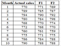
Compute the MAD and MSE as shown below in the table:

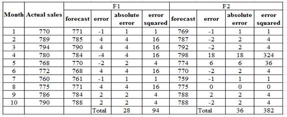
Compute the Mean absolute deviation (MAD) for the forecasting method F₁ as shown below

$MAD=\frac{{\displaystyle \sum \left|error\right|}}{n}$

Substitute the value of ${\displaystyle \sum \left|error\right|}=28$ and the value of $n=10$ to obtain the Mean absolute deviation (MAD)

$MAD=\frac{28}{10}=\underset{\_}{2.8}$

Compute the Mean squared error (MSE) for the forecasting method F₁ as shown below

$MSE=\frac{{\displaystyle \sum \left|erro{r}^2\right|}}{n-1}$

Substitute the value of ${\displaystyle \sum \left|erro{r}^2\right|}=94$ and the value of $n=10$ to obtain the Mean squared error (MSE)

$MSE=\frac{94}{10-1}=\underset{\_}{10.44}$

Compute the Mean absolute deviation (MAD) for the forecasting method F₂ as shown below

$MAD=\frac{{\displaystyle \sum \left|error\right|}}{n}$

Substitute the value of ${\displaystyle \sum \left|error\right|}=36$ and the value of $n=10$ to obtain the Mean absolute deviation (MAD)

$MAD=\frac{36}{10}=\underset{\_}{3.6}$

Compute the Mean squared error (MSE) for the forecasting method F₂ as shown below

$MSE=\frac{{\displaystyle \sum \left|erro{r}^2\right|}}{n-1}$

Substitute the value of ${\displaystyle \sum \left|erro{r}^2\right|}=382$ and the value of $n=10$ to obtain the Mean squared error (MSE)

$MSE=\frac{382}{10-1}=\underset{\_}{42.44}$

The first forecasting method F₁ gives both a low value of MAD as well as MSE compared to the second forecasting method F₂

Summary Introduction

To compute: Mean Absolute Percentage Error for both the forecasts F₁ and F₂ as shown below.

Introduction: Forecasting is the planning process that helps to predict the future demand using present or past data. It uses certain assumptions based the knowledge and experience of the management.

Explanation of Solution

Determine MAPE for both the forecasts:

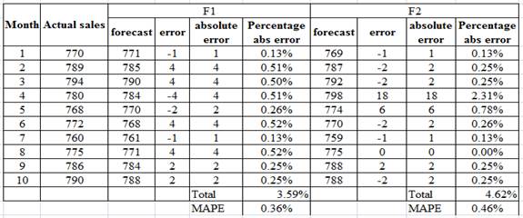
The Mean absolute percentage error is lower at 0.36% for the first forecasting method F₁ compared to MAPE of 0.46% for the second forecasting method F₂

Summary Introduction

To prepare: A naïve forecast.

Introduction: Forecasting is the planning process that helps to predict the future demand using present or past data. It uses certain assumptions based the knowledge and experience of the management.

Explanation of Solution

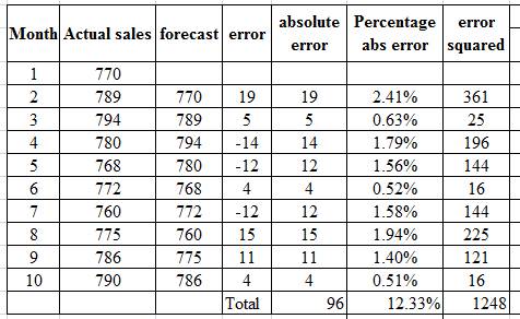
Determine MAD and MSE using a naïve forecast:

Use the naïve method for forecasting as shown below.

(i)

Compute the Mean absolute deviation (MAD) for the naïve forecasting method as shown below

$MAD=\frac{{\displaystyle \sum \left|error\right|}}{n}$

Substitute the value of ${\displaystyle \sum \left|error\right|}=96$ and the value of $n=9$ to obtain the Mean absolute deviation (MAD)

$MAD=\frac{96}{9}=\underset{\_}{10.67}$

(ii)

Compute the Mean squared error (MSE) for the naïve forecasting method as shown below

$MSE=\frac{{\displaystyle \sum \left|erro{r}^2\right|}}{n-1}$

Substitute the value of ${\displaystyle \sum \left|erro{r}^2\right|}=1,248$ and the value of $n=9$ to obtain the Mean squared error (MSE)

$MSE=\frac{1,248}{9-1}=\underset{\_}{156}$

(iii)

Compute the tracking signal on the 10^th month as shown below.

First compute the cumulative forecast error (CFE) as shown below

12.49=

$CFE=19+5-14-12+4-12+15+11+4=20$

Compute the tracking signal (TS) by dividing the cumulative forecast error by MAD as shown below.

$TS=\frac{20}{10.67}=\underset{\_}{1.87}$

(iv)

Given the Mean Squared Error is 156, the standard deviation σ is 12.49

The two sigma control limits are +2×12.49=24.98 and -2×12.49=–24.98

Since the tracking signal 1.87 falls between +24.98 and –24.98, the forecasting process is in control

The comparison of the naïve method with the other two forecasting methods is shown below.

Obviously the naïve method compares very poorly with the other two methods F₁ and F₂, since both the Mean Absolute Deviation (MAD) and Mean Squared Error (MSE) are worse than the other two methods.