Elementary Statistics ( 3rd International Edition ) Isbn:9781260092561
3rd Edition
ISBN: 9781259969454
Author: William Navidi Prof.; Barry Monk Professor
Publisher: McGraw-Hill Education
expand_more
expand_more
format_list_bulleted
Videos
Textbook Question
Chapter 2.4, Problem 14E
Food expenditures: Both of the following time-series plots present the percentage of income spent on food by U.S. residents for the years 1998 through 2014. (Source: U.S. Department of Agriculture)
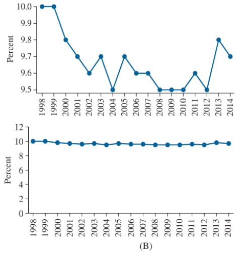
Which of the following statements is more accurate, and why?
(i) The percentage of income spent on food decreased considerably between 1998 and 2014.
(ii) The percentage of income spent on food decreased slightly between 1998 and 2014.
Expert Solution & Answer
Want to see the full answer?
Check out a sample textbook solution
Students have asked these similar questions
Suppose that 80% of athletes at a certain college graduate. You randomly select eight athletes. What’s the chance that at most 7 of them graduate?
Suppose that you flip a fair coin four times. What’s the chance of getting at least one head?
Suppose that the chance that an elementary student eats hot lunch is 30 percent. What’s the chance that, among 20 randomly selected students, between 6 and 8 students eat hot lunch (inclusive)?
Chapter 2 Solutions
Elementary Statistics ( 3rd International Edition ) Isbn:9781260092561
Ch. 2.1 - In Exercises 5-8, fill in each blank with the...Ch. 2.1 - In Exercises 5-8, fill in each blank with the...Ch. 2.1 - In Exercises 5-8, fill in each blank with the...Ch. 2.1 - In Exercises 5-8, fill in each blank with the...Ch. 2.1 - In Exercises 9—12, determine whether the...Ch. 2.1 - In Exercises 9—12, determine whether the...Ch. 2.1 - In Exercises 9—12, determine whether the...Ch. 2.1 - In Exercises 9—12, determine whether the...Ch. 2.1 - The following bar graph presents the average...Ch. 2.1 - The most common blood typing system divides human...
Ch. 2.1 - Following is a pie chart that presents the...Ch. 2.1 - Government spending: The following pie chart...Ch. 2.1 - U.S. population: The following side-by-side bar...Ch. 2.1 - Super Bowl: The following side-by-side bar graph...Ch. 2.1 - Smartphone sales: The following frequency...Ch. 2.1 - Popular video games: The following frequency...Ch. 2.1 - More smartphones: Using the data in Exercise 19:...Ch. 2.1 - More video games: Using the data in Exercise 20:...Ch. 2.1 - Hospital admissions: The following frequency...Ch. 2.1 - World population: Following are the populations of...Ch. 2.1 - Ages of video garners: The Nielsen Company...Ch. 2.1 - How secure is your job? In a survey, employed...Ch. 2.1 - Back up your data: In a survey commissioned by the...Ch. 2.1 - Education levels: The following frequency...Ch. 2.1 - Twitter followers: The following frequency...Ch. 2.1 - Music sales: The following frequency distribution...Ch. 2.1 - Keeping up with the Kardashians: The following...Ch. 2.1 - Bought a new car lately? The following table...Ch. 2.1 - Bought a new- truck lately? The following table...Ch. 2.1 - Happy Halloween: The following table presents...Ch. 2.1 - Native languages: The following frequency...Ch. 2.1 - Proportion of females: Following are the...Ch. 2.2 - Prob. 5ECh. 2.2 - In Exercises 5—8, fill in each blank with the...Ch. 2.2 - In Exercises 5—8, fill in each blank with the...Ch. 2.2 - In Exercises 5—8, fill in each blank with the...Ch. 2.2 - In Exercises 9—12, determine whether the...Ch. 2.2 - In Exercises 9—12, determine whether the...Ch. 2.2 - In Exercises 9—12, determine whether the...Ch. 2.2 - In Exercises 9—12, determine whether the...Ch. 2.2 - In Exercises 13—16, classify the histogram as...Ch. 2.2 - In Exercises 13—16, classify the histogram as...Ch. 2.2 - In Exercises 13—16, classify the histogram as...Ch. 2.2 - In Exercises 13—16, classify the histogram as...Ch. 2.2 - In Exercises 17 and 18, classify the histogram as...Ch. 2.2 - In Exercises 17 and 18, classify the histogram as...Ch. 2.2 - Student heights: The following frequency histogram...Ch. 2.2 - Trained rats: Forty rats were trained to run a...Ch. 2.2 - Cholesterol: The following histogram shows the...Ch. 2.2 - Blood pressure: The following histogram shows the...Ch. 2.2 - Olympic athletes: The following frequency...Ch. 2.2 - Hows the weather? The following relative frequency...Ch. 2.2 - Skewed which way? For which of the following data...Ch. 2.2 - Skewed which way? For which of the following data...Ch. 2.2 - Batting average: The following frequency...Ch. 2.2 - Batting average: The following frequency...Ch. 2.2 - Time spent playing video games: A sample of 200...Ch. 2.2 - Murder, she wrote: The following frequency...Ch. 2.2 - BMW prices: The following table presents the...Ch. 2.2 - Geysers: The geyser Old Faithful in Yellowstone...Ch. 2.2 - Hail to the chief: There have been 58 presidential...Ch. 2.2 - Internet radio: The following table presents the...Ch. 2.2 - Brothers and sisters: Thirty students in a...Ch. 2.2 - Cough, cough: The following table presents the...Ch. 2.2 - Prob. 37ECh. 2.2 - Prob. 38ECh. 2.2 - Prob. 39ECh. 2.2 - Prob. 40ECh. 2.2 - Frequency polygon: Using the data in Exercise 29:...Ch. 2.2 - Prob. 42ECh. 2.2 - Ogive: Using the data in Exercise 27: Compute the...Ch. 2.2 - Ogive: Using the data in Exercise 28: Compute the...Ch. 2.2 - Ogive: Using the data in Exercise 29: Compute the...Ch. 2.2 - Prob. 46ECh. 2.2 - Prob. 47ECh. 2.2 - Prob. 48ECh. 2.2 - Prob. 49ECh. 2.2 - Prob. 50ECh. 2.2 - Prob. 51ECh. 2.2 - Prob. 52ECh. 2.2 - Frequencies and relative frequencies: The...Ch. 2.3 - In Exercises 3—6, fill in each blank with the...Ch. 2.3 - In Exercises 3—6, fill in each blank with the...Ch. 2.3 - In Exercises 3—6, fill in each blank with the...Ch. 2.3 - In Exercises 3—6, fill in each blank with the...Ch. 2.3 - Prob. 7ECh. 2.3 - In Exercises 7—10, determine whether the...Ch. 2.3 - In Exercises 7—10, determine whether the...Ch. 2.3 - In Exercises 7—10, determine whether the...Ch. 2.3 - Construct a stem-and-leaf plot for the following...Ch. 2.3 - Construct a stem-and-leaf plot for the following...Ch. 2.3 - List the data in the following stem-and-leaf plot....Ch. 2.3 - List the data in the following stein-and-leaf...Ch. 2.3 - Construct a dotplot for the data in Exercise 11.Ch. 2.3 - Prob. 16ECh. 2.3 - BMW prices: The following table presents the...Ch. 2.3 - Hows the weather? The following table presents the...Ch. 2.3 - Air pollution: The following table presents...Ch. 2.3 - Technology salaries: The following table presents...Ch. 2.3 - Tennis and golf: Following are the ages of the...Ch. 2.3 - Pass the popcorn: Following are the running times...Ch. 2.3 - More weather: Construct a dotplot for the data in...Ch. 2.3 - Prob. 24ECh. 2.3 - Looking for a job: The following table presents...Ch. 2.3 - Prob. 26ECh. 2.3 - Military spending: The following table presents...Ch. 2.3 - Prob. 28ECh. 2.3 - Dining out: The following time-series plot...Ch. 2.3 - Prob. 30ECh. 2.3 - Prob. 31ECh. 2.3 - More gold: The following time series plot presents...Ch. 2.3 - Prob. 33ECh. 2.3 - Prob. 34ECh. 2.3 - Vote: The following time-series plot presents the...Ch. 2.3 - Arctic ice sheet: The following table presents the...Ch. 2.3 - Prob. 37ECh. 2.4 - In Exercises 3 and 4, fill in each blank with the...Ch. 2.4 - In Exercises 3 and 4, fill in each blank with the...Ch. 2.4 - CD sales decline: Sales of CDs have been declining...Ch. 2.4 - Music sales: The following time-series plot and...Ch. 2.4 - Stock market prices: The Dow Jones Industrial...Ch. 2.4 - Save your money: In 2007, U.S. residents saved...Ch. 2.4 - Ill take mine with mustard: The following bar...Ch. 2.4 - Stream or download? The following bar graph...Ch. 2.4 - Female senators: Of the 100 members of the United...Ch. 2.4 - Age at marriage: Data compiled by the U.S. Census...Ch. 2.4 - College degrees: Both of the following time-series...Ch. 2.4 - Food expenditures: Both of the following...Ch. 2.4 - Prob. 15ECh. 2 - Following is the list of letter grades for...Ch. 2 - Prob. 2CQCh. 2 - Construct a frequency bar graph for the data in...Ch. 2 - Prob. 4CQCh. 2 - Prob. 5CQCh. 2 - Prob. 6CQCh. 2 - Prob. 7CQCh. 2 - Prob. 8CQCh. 2 - Prob. 9CQCh. 2 - Prob. 10CQCh. 2 - Following are the prices (in dollars) for a sample...Ch. 2 - Prob. 12CQCh. 2 - Prob. 13CQCh. 2 - Prob. 14CQCh. 2 - Prob. 15CQCh. 2 - Trust your doctor: The General Social Survey...Ch. 2 - Internet browsers: The following relative...Ch. 2 - Prob. 3RECh. 2 - Prob. 4RECh. 2 - Prob. 5RECh. 2 - House freshmen: Newly elected members of the U.S....Ch. 2 - More freshmen: For the data in Exercise 6:...Ch. 2 - Royalty: Following are the ages at death for all...Ch. 2 - Prob. 9RECh. 2 - Prob. 10RECh. 2 - Prob. 11RECh. 2 - Prob. 12RECh. 2 - Prob. 13RECh. 2 - Prob. 14RECh. 2 - Prob. 15RECh. 2 - Explain why the frequency bar graph and the...Ch. 2 - Prob. 2WAICh. 2 - Prob. 3WAICh. 2 - Prob. 4WAICh. 2 - Prob. 5WAICh. 2 - In the chapter introduction, we presented gas...Ch. 2 - In the chapter introduction, we presented gas...Ch. 2 - In the chapter introduction, we presented gas...Ch. 2 - Prob. 4CSCh. 2 - In the chapter introduction, we presented gas...Ch. 2 - Prob. 6CSCh. 2 - In the chapter introduction, we presented gas...Ch. 2 - Prob. 8CSCh. 2 - In the chapter introduction, we presented gas...
Knowledge Booster


Learn more about
Need a deep-dive on the concept behind this application? Look no further. Learn more about this topic, statistics and related others by exploring similar questions and additional content below.Similar questions
- Bob’s commuting times to work are varied. He makes it to work on time 80 percent of the time. On 12 randomly selected trips to work, what’s the chance that Bob makes it on time at least 10 times?arrow_forwardYour chance of winning a small prize in a scratch-off ticket is 10 percent. You buy five tickets. What’s the chance you will win at least one prize?arrow_forwardSuppose that 60 percent of families own a pet. You randomly sample four families. What is the chance that two or three of them own a pet?arrow_forward
- If 40 percent of university students purchase their textbooks online, in a random sample of five students, what’s the chance that exactly one of them purchased their textbooks online?arrow_forwardA stoplight is green 40 percent of the time. If you stop at this light eight random times, what is the chance that it’s green exactly five times?arrow_forwardIf 10 percent of the parts made by a certain company are defective and have to be remade, what is the chance that a random sample of four parts has one that is defective?arrow_forward
- Question 4 Fourteen individuals were given a complex puzzle to complete. The times in seconds was recorded for their first and second attempts and the results provided below: 1 2 3 first attempt 172 255 second attempt 70 4 5 114 248 218 194 270 267 66 6 7 230 219 341 174 8 10 9 210 261 347 218 200 281 199 308 268 243 236 300 11 12 13 14 140 302 a. Calculate a 95% confidence interval for the mean time taken by each individual to complete the (i) first attempt and (ii) second attempt. [la] b. Test the hypothesis that the difference between the two mean times for both is 100 seconds. Use the 5% level of significance. c. Subsequently, it was learnt that the times for the second attempt were incorrecly recorded and that each of the values is 50 seconds too large. What, if any, difference does this make to the results of the test done in part (b)? Show all steps for the hypothesis testarrow_forwardQuestion 3 3200 students were asked about the importance of study groups in successfully completing their courses. They were asked to provide their current majors as well as their opinion. The results are given below: Major Opinion Psychology Sociology Economics Statistics Accounting Total Agree 144 183 201 271 251 1050 Disagree 230 233 254 227 218 1162 Impartial 201 181 196 234 176 988 Total 575 597 651 732 645 3200 a. State both the null and alternative hypotheses. b. Provide the decision rule for making this decision. Use an alpha level of 5%. c. Show all of the work necessary to calculate the appropriate statistic. | d. What conclusion are you allowed to draw? c. Would your conclusion change at the 10% level of significance? f. Confirm test results in part (c) using JASP. Note: All JASP input files and output tables should be providedarrow_forwardQuestion 1 A tech company has acknowledged the importance of having records of all meetings conducted. The meetings are very fast paced and requires equipment that is able to capture the information in the shortest possible time. There are two options, using a typewriter or a word processor. Fifteen administrative assistants are selected and the amount of typing time in hours was recorded. The results are given below: 1 2 3 4 5 6 7 8 9 10 11 12 13 14 15 typewriter 8.0 6.5 5.0 6.7 7.8 8.5 7.2 5.7 9.2 5.7 6.5 word processor 7.2 5.7 8.3 7.5 9.2 7.2 6.5 7.0 6.9 34 7.0 6.9 8.8 6.7 8.8 9.4 8.6 5.5 7.2 8.4 a. Test the hypothesis that the mean typing time in hours for typewriters is less than 7.0. Use the 1% level of significance. b. Construct a 90% confidence interval for the difference in mean typing time in hours, where a difference is equal to the typing time in hours of word processors minus typing time in hours of typewriter. c. Using the 5% significance level, determine whether there is…arrow_forward
- Illustrate 2/7×4/5 using a rectangular region. Explain your work. arrow_forwardWrite three other different proportions equivalent to the following using the same values as in the given proportion 3 foot over 1 yard equals X feet over 5 yardsarrow_forward2. An experiment is set up to test the effectiveness of a new drug for balancing people's mood. The table below contains the results of the patients before and after taking the drug. The possible scores are the integers from 0 to 10, where 0 indicates a depressed mood and 10 indicates and elated mood. Patient Before After 1 4 4 2 3 3 3 6 4 4 1 2 5 6 5 6 1 3 7 4 7 8 6 9 1 4 10 5 4 Assuming the differences of the observations to be symmetric, but not normally distributed, investigate the effectiveness of the drug at the 5% significance level. [4 Marks]arrow_forward
arrow_back_ios
SEE MORE QUESTIONS
arrow_forward_ios
Recommended textbooks for you
 Glencoe Algebra 1, Student Edition, 9780079039897...AlgebraISBN:9780079039897Author:CarterPublisher:McGraw Hill
 Functions and Change: A Modeling Approach to Coll...AlgebraISBN:9781337111348Author:Bruce Crauder, Benny Evans, Alan NoellPublisher:Cengage Learning
 Holt Mcdougal Larson Pre-algebra: Student Edition...AlgebraISBN:9780547587776Author:HOLT MCDOUGALPublisher:HOLT MCDOUGAL
Glencoe Algebra 1, Student Edition, 9780079039897...
Algebra
ISBN:9780079039897
Author:Carter
Publisher:McGraw Hill
Functions and Change: A Modeling Approach to Coll...
Algebra
ISBN:9781337111348
Author:Bruce Crauder, Benny Evans, Alan Noell
Publisher:Cengage Learning
Holt Mcdougal Larson Pre-algebra: Student Edition...
Algebra
ISBN:9780547587776
Author:HOLT MCDOUGAL
Publisher:HOLT MCDOUGAL
What Are Research Ethics?; Author: HighSchoolScience101;https://www.youtube.com/watch?v=nX4c3V23DZI;License: Standard YouTube License, CC-BY
What is Ethics in Research - ethics in research (research ethics); Author: Chee-Onn Leong;https://www.youtube.com/watch?v=W8Vk0sXtMGU;License: Standard YouTube License, CC-BY