
Concept explainers
Videos
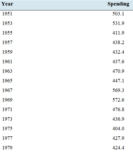
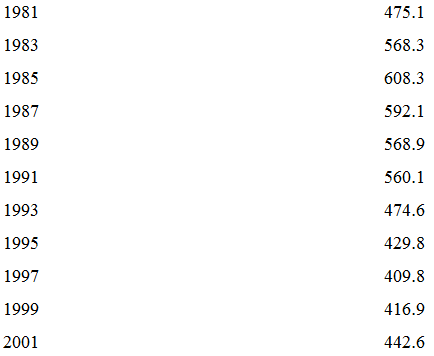
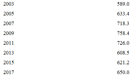
Military spending: The following table presents the amount spent, in billions of dollars, on national defense by the U.S. government every other year for the years 1951 through 2017. The amounts are adjusted for inflation, and represent 2017 dollars.
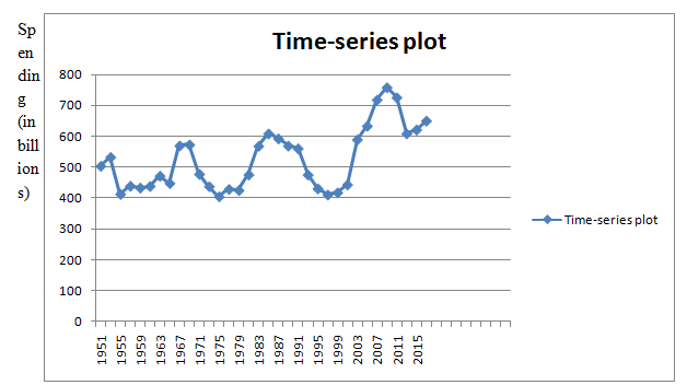
- Construct a time-series plot for these data.
- The plot covers seven decades, from the 1950s through the period 2010—2017. During which of these decades did national defense spending increase, and during which decades did it decrease?
- The United States fought in the Korean War, which ended in 1953. What effect did the end of the war have on military spending after 1953?
- During the period 1965—1963, the United States steadily increased the number of troops in Vietnam from 23,000 at the beginning of 1965 to 537.000 at the end of 1968.
Beginning in 1969, the number of Americans in Vietnam was steadily reduced, with the last of them leaving in 1975. How is this reflected in the national defense spending from 1965 to 1975?
a.
To construct:A time-series plot of the given data.
Explanation of Solution
Given information:
The dataset:
| Year | Spending |
| 1951 | 503.1 |
| 1953 | 531.9 |
| 1955 | 411.9 |
| 1957 | 438.2 |
| 1959 | 432.4 |
| 1961 | 437.6 |
| 1963 | 470.9 |
| 1965 | 447.1 |
| 1967 | 569.3 |
| 1969 | 572.6 |
| 1971 | 476.8 |
| 1973 | 436.9 |
| 1975 | 404.0 |
| 1977 | 427.9 |
| 1979 | 424.4 |
| 1981 | 475.1 |
| 1983 | 568.3 |
| 1985 | 608.3 |
| 1987 | 592.1 |
| 1989 | 568.9 |
| 1991 | 560.1 |
| 1993 | 474.6 |
| 1995 | 429.8 |
| 1997 | 409.8 |
| 1999 | 416.9 |
| 2001 | 442.6 |
| 2003 | 589.0 |
| 2005 | 633.4 |
| 2007 | 718.3 |
| 2009 | 758.4 |
| 2011 | 726.0 |
| 2013 | 608.5 |
| 2015 | 621.2 |
| 2017 | 650.0 |
Graph:
A time-series plot for the given data is given by
b.
To find:The decade during which the national defence spending increasing and the decade during which the national defence spending increasing.
Answer to Problem 27E
The trend in the vacancy rate during the time period from 2012 to 2015 is decreasing.
Explanation of Solution
Solution:
A time-series plot for the given data is given by
From the time-series plot, we can see that during 1960s, 1980s and 2000s, the national defence spending is increasing and during 1950s, 1970s, 1990s and 2010s, the national defence spending is decreasing
Hence,
Increased decade: 1960s, 1980s and 2000s
Decreased decade: 1950s, 1970s, 1990s and 2010s.
c.
To find: The effects of the end of the war have on military spending after 1953.
Answer to Problem 27E
The effects of the end of the war have on military spending after 1953 is that it caught a big decrease.
Explanation of Solution
Solution:
A time-series plot for the given data is given by
From the time-series plot, we can see that after 1953, there was causing a big decrease in the military spending. The military spending was falling from 531.9 to 411.9 during 1953-1955.
Hence, the effects of the end of the war have on military spending after 1953 is that there caused a big decrease.
d.
To explain: The reflection in the national defence spending from 1965 to 1975.
Answer to Problem 27E
The national defence spending is increased from 1965 to 1969 and then decreased from 1969 to 1975.
Explanation of Solution
Given information: The following table presents the amount spent, in billions of dollars, on national defence by the U.S. government every other year for the years 1951 through 2017. The amounts are adjusted for inflation, and represent 2017 dollars.
| Year | Spending |
| 1951 | 503.1 |
| 1953 | 531.9 |
| 1955 | 411.9 |
| 1957 | 438.2 |
| 1959 | 432.4 |
| 1961 | 437.6 |
| 1963 | 470.9 |
| 1965 | 447.1 |
| 1967 | 569.3 |
| 1969 | 572.6 |
| 1971 | 476.8 |
| 1973 | 436.9 |
| 1975 | 404.0 |
| 1977 | 427.9 |
| 1979 | 424.4 |
| 1981 | 475.1 |
| 1983 | 568.3 |
| 1985 | 608.3 |
| 1987 | 592.1 |
| 1989 | 568.9 |
| 1991 | 560.1 |
| 1993 | 474.6 |
| 1995 | 429.8 |
| 1997 | 409.8 |
| 1999 | 416.9 |
| 2001 | 442.6 |
| 2003 | 589.0 |
| 2005 | 633.4 |
| 2007 | 718.3 |
| 2009 | 758.4 |
| 2011 | 726.0 |
| 2013 | 608.5 |
| 2015 | 621.2 |
| 2017 | 650.0 |
During the period 1965-1968, the United States steadily increased the number of troops in Vietnam from 23,000 at the beginning of 1965 to 537,000 at the end of 1968. Beginning in 1969, the number of Americans in Vietnam was steadily reduced, with the last of themleaving in 1975.
A time-series plot for the given data is given by
From 1965 to 1975, the national defence spending is increasing from 1965 to 1969 and then decreasing from 1969 to 1975.
Hence, the national defence spending is increased from 1965 to 1969 and then decreased from 1969 to 1975.
Want to see more full solutions like this?
Chapter 2 Solutions
Elementary Statistics ( 3rd International Edition ) Isbn:9781260092561


- Question 6. You collect daily data for the stock of a company Z over the past 4 months (i.e. 80 days) and calculate the log-returns (yk)/(-1. You want to build a CRR model for the evolution of the stock. The expected value and standard deviation of the log-returns are y = 0.06 and Sy 0.1. The money market interest rate is r = 0.04. Determine the risk-neutral probability of the model.arrow_forwardSeveral markets (Japan, Switzerland) introduced negative interest rates on their money market. In this problem, we will consider an annual interest rate r < 0. We consider a stock modeled by an N-period CRR model where each period is 1 year (At = 1) and the up and down factors are u and d. (a) We consider an American put option with strike price K and expiration T. Prove that if <0, the optimal strategy is to wait until expiration T to exercise.arrow_forwardWe consider an N-period CRR model where each period is 1 year (At = 1), the up factor is u = 0.1, the down factor is d = e−0.3 and r = 0. We remind you that in the CRR model, the stock price at time tn is modeled (under P) by Sta = So exp (μtn + σ√AtZn), where (Zn) is a simple symmetric random walk. (a) Find the parameters μ and σ for the CRR model described above. (b) Find P Ste So 55/50 € > 1). StN (c) Find lim P 804-N (d) Determine q. (You can use e- 1 x.) Ste (e) Find Q So (f) Find lim Q 004-N StN Soarrow_forward
- In this problem, we consider a 3-period stock market model with evolution given in Fig. 1 below. Each period corresponds to one year. The interest rate is r = 0%. 16 22 28 12 16 12 8 4 2 time Figure 1: Stock evolution for Problem 1. (a) A colleague notices that in the model above, a movement up-down leads to the same value as a movement down-up. He concludes that the model is a CRR model. Is your colleague correct? (Explain your answer.) (b) We consider a European put with strike price K = 10 and expiration T = 3 years. Find the price of this option at time 0. Provide the replicating portfolio for the first period. (c) In addition to the call above, we also consider a European call with strike price K = 10 and expiration T = 3 years. Which one has the highest price? (It is not necessary to provide the price of the call.) (d) We now assume a yearly interest rate r = 25%. We consider a Bermudan put option with strike price K = 10. It works like a standard put, but you can exercise it…arrow_forwardIn this problem, we consider a 2-period stock market model with evolution given in Fig. 1 below. Each period corresponds to one year (At = 1). The yearly interest rate is r = 1/3 = 33%. This model is a CRR model. 25 15 9 10 6 4 time Figure 1: Stock evolution for Problem 1. (a) Find the values of up and down factors u and d, and the risk-neutral probability q. (b) We consider a European put with strike price K the price of this option at time 0. == 16 and expiration T = 2 years. Find (c) Provide the number of shares of stock that the replicating portfolio contains at each pos- sible position. (d) You find this option available on the market for $2. What do you do? (Short answer.) (e) We consider an American put with strike price K = 16 and expiration T = 2 years. Find the price of this option at time 0 and describe the optimal exercising strategy. (f) We consider an American call with strike price K ○ = 16 and expiration T = 2 years. Find the price of this option at time 0 and describe…arrow_forward2.2, 13.2-13.3) question: 5 point(s) possible ubmit test The accompanying table contains the data for the amounts (in oz) in cans of a certain soda. The cans are labeled to indicate that the contents are 20 oz of soda. Use the sign test and 0.05 significance level to test the claim that cans of this soda are filled so that the median amount is 20 oz. If the median is not 20 oz, are consumers being cheated? Click the icon to view the data. What are the null and alternative hypotheses? OA. Ho: Medi More Info H₁: Medi OC. Ho: Medi H₁: Medi Volume (in ounces) 20.3 20.1 20.4 Find the test stat 20.1 20.5 20.1 20.1 19.9 20.1 Test statistic = 20.2 20.3 20.3 20.1 20.4 20.5 Find the P-value 19.7 20.2 20.4 20.1 20.2 20.2 P-value= (R 19.9 20.1 20.5 20.4 20.1 20.4 Determine the p 20.1 20.3 20.4 20.2 20.3 20.4 Since the P-valu 19.9 20.2 19.9 Print Done 20 oz 20 oz 20 oz 20 oz ce that the consumers are being cheated.arrow_forward
- T Teenage obesity (O), and weekly fast-food meals (F), among some selected Mississippi teenagers are: Name Obesity (lbs) # of Fast-foods per week Josh 185 10 Karl 172 8 Terry 168 9 Kamie Andy 204 154 12 6 (a) Compute the variance of Obesity, s²o, and the variance of fast-food meals, s², of this data. [Must show full work]. (b) Compute the Correlation Coefficient between O and F. [Must show full work]. (c) Find the Coefficient of Determination between O and F. [Must show full work]. (d) Obtain the Regression equation of this data. [Must show full work]. (e) Interpret your answers in (b), (c), and (d). (Full explanations required). Edit View Insert Format Tools Tablearrow_forwardThe average miles per gallon for a sample of 40 cars of model SX last year was 32.1, with a population standard deviation of 3.8. A sample of 40 cars from this year’s model SX has an average of 35.2 mpg, with a population standard deviation of 5.4. Find a 99 percent confidence interval for the difference in average mpg for this car brand (this year’s model minus last year’s).Find a 99 percent confidence interval for the difference in average mpg for last year’s model minus this year’s. What does the negative difference mean?arrow_forwardA special interest group reports a tiny margin of error (plus or minus 0.04 percent) for its online survey based on 50,000 responses. Is the margin of error legitimate? (Assume that the group’s math is correct.)arrow_forward
- Suppose that 73 percent of a sample of 1,000 U.S. college students drive a used car as opposed to a new car or no car at all. Find an 80 percent confidence interval for the percentage of all U.S. college students who drive a used car.What sample size would cut this margin of error in half?arrow_forwardYou want to compare the average number of tines on the antlers of male deer in two nearby metro parks. A sample of 30 deer from the first park shows an average of 5 tines with a population standard deviation of 3. A sample of 35 deer from the second park shows an average of 6 tines with a population standard deviation of 3.2. Find a 95 percent confidence interval for the difference in average number of tines for all male deer in the two metro parks (second park minus first park).Do the parks’ deer populations differ in average size of deer antlers?arrow_forwardSuppose that you want to increase the confidence level of a particular confidence interval from 80 percent to 95 percent without changing the width of the confidence interval. Can you do it?arrow_forward

 College AlgebraAlgebraISBN:9781305115545Author:James Stewart, Lothar Redlin, Saleem WatsonPublisher:Cengage Learning