Concept explainers
Videos
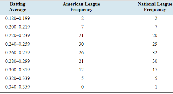
Batting average: The following frequency distribution presents the batting averages of Major League Baseball players in both the American League and the National League who had 300 or more plate appearances during a recent season.
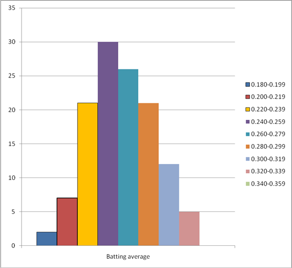
- Construct a frequency histogram for the American League.
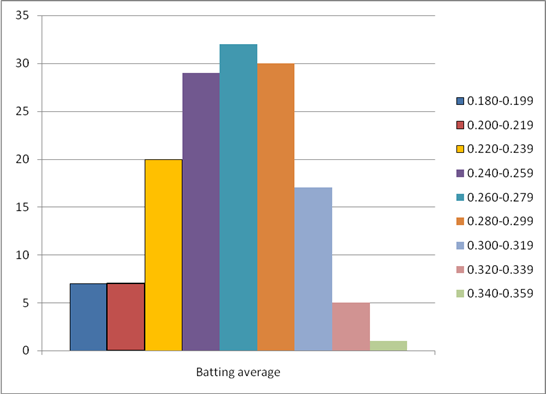
- Construct a frequency histogram for the National League.
- Construct a relative frequency distribution for the American League.
- Construct a relative frequency distribution for the National League.
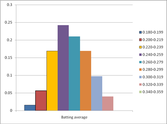
- Construct a relative frequency histogram for the American League.
- Construct a relative frequency histogram for the National League.
- What percentage of American League players had batting averages of 0.300 or more?
- What percentage of National League players had batting averages of 0.300 or more?
- Compare the relative frequency histograms. What is the main difference between the distributions of batting averages in the two leagues?
a.
To construct: A frequency histogram for American League.
Explanation of Solution
Given information:The following frequency distribution presents the batting averages of Major League Baseball players in both the American League and the National League who had 300 or more plate appearances during a recent season.
| Batting average | American LeagueFrequency | National LeagueFrequency |
| 0.180-0.199 | 2 | 2 |
| 0.200-0.219 | 7 | 7 |
| 0.220-0.239 | 21 | 20 |
| 0.240-0.259 | 30 | 29 |
| 0.260-0.279 | 26 | 32 |
| 0.280-0.299 | 21 | 30 |
| 0.300-0.319 | 12 | 17 |
| 0.320-0.339 | 5 | 5 |
| 0.340-0.359 | 0 | 1 |
Definition used: Histograms based on frequency distributions are called frequency histogram.
Solution:
The following frequency distribution presents the batting averages of Major League Baseball players in the American Leaguewho had 300 or more plate appearances during a recent season.
| Batting average | American LeagueFrequency |
| 0.180-0.199 | 2 |
| 0.200-0.219 | 7 |
| 0.220-0.239 | 21 |
| 0.240-0.259 | 30 |
| 0.260-0.279 | 26 |
| 0.280-0.299 | 21 |
| 0.300-0.319 | 12 |
| 0.320-0.339 | 5 |
| 0.340-0.359 | 0 |
The frequency histogram for American League is given by
b.
To construct: A frequency histogram for National League.
Explanation of Solution
Given information:The following frequency distribution presents the batting averages of Major League Baseball players in both the American League and the National League who had 300 or more plate appearances during a recent season.
| Batting average | American LeagueFrequency | National LeagueFrequency |
| 0.180-0.199 | 2 | 2 |
| 0.200-0.219 | 7 | 7 |
| 0.220-0.239 | 21 | 20 |
| 0.240-0.259 | 30 | 29 |
| 0.260-0.279 | 26 | 32 |
| 0.280-0.299 | 21 | 30 |
| 0.300-0.319 | 12 | 17 |
| 0.320-0.339 | 5 | 5 |
| 0.340-0.359 | 0 | 1 |
Definition used: Histograms based on frequency distributions are called frequency histogram.
Solution:
The following frequency distribution presents the batting averages of Major League Baseball players in the American Leaguewho had 300 or more plate appearances during a recent season.
| Batting average | National LeagueFrequency |
| 0.180-0.199 | 2 |
| 0.200-0.219 | 7 |
| 0.220-0.239 | 20 |
| 0.240-0.259 | 29 |
| 0.260-0.279 | 32 |
| 0.280-0.299 | 30 |
| 0.300-0.319 | 17 |
| 0.320-0.339 | 5 |
| 0.340-0.359 | 1 |
The frequency histogram for American League is given by
c.
To construct: A relative frequency distribution for American League.
Explanation of Solution
Given information:The following frequency distribution presents the batting averages of Major League Baseball players in both the American League and the National League who had 300 or more plate appearances during a recent season.
| Batting average | American LeagueFrequency | National LeagueFrequency |
| 0.180-0.199 | 2 | 2 |
| 0.200-0.219 | 7 | 7 |
| 0.220-0.239 | 21 | 20 |
| 0.240-0.259 | 30 | 29 |
| 0.260-0.279 | 26 | 32 |
| 0.280-0.299 | 21 | 30 |
| 0.300-0.319 | 12 | 17 |
| 0.320-0.339 | 5 | 5 |
| 0.340-0.359 | 0 | 1 |
Formula used:
Solution:
From the given table,
The sum of all frequency for American League is
The table of relative frequency is given by
| Batting average | American LeagueFrequency | American LeagueRelative frequency |
| 0.180-0.199 | 2 | |
| 0.200-0.219 | 7 | |
| 0.220-0.239 | 21 | |
| 0.240-0.259 | 30 | |
| 0.260-0.279 | 26 | |
| 0.280-0.299 | 21 | |
| 0.300-0.319 | 12 | |
| 0.320-0.339 | 5 | |
| 0.340-0.359 | 0 |
The relative frequency for the American League is given by
| Batting average | American LeagueRelative frequency |
| 0.180-0.199 | 0.016 |
| 0.200-0.219 | 0.056 |
| 0.220-0.239 | 0.169 |
| 0.240-0.259 | 0.242 |
| 0.260-0.279 | 0.210 |
| 0.280-0.299 | 0.169 |
| 0.300-0.319 | 0.097 |
| 0.320-0.339 | 0.040 |
| 0.340-0.359 | 0.000 |
d.
To construct: A relative frequency distribution for National League.
Explanation of Solution
Given information:The following frequency distribution presents the batting averages of Major League Baseball players in both the American League and the National League who had 300 or more plate appearances during a recent season.
| Batting average | American LeagueFrequency | National LeagueFrequency |
| 0.180-0.199 | 2 | 2 |
| 0.200-0.219 | 7 | 7 |
| 0.220-0.239 | 21 | 20 |
| 0.240-0.259 | 30 | 29 |
| 0.260-0.279 | 26 | 32 |
| 0.280-0.299 | 21 | 30 |
| 0.300-0.319 | 12 | 17 |
| 0.320-0.339 | 5 | 5 |
| 0.340-0.359 | 0 | 1 |
Formula used:
Solution:
From the given table,
The sum of all frequency for National League is
The table of relative frequency is given by
| Batting average | National LeagueFrequency | National LeagueRelative frequency |
| 0.180-0.199 | 2 | |
| 0.200-0.219 | 7 | |
| 0.220-0.239 | 20 | |
| 0.240-0.259 | 29 | |
| 0.260-0.279 | 32 | |
| 0.280-0.299 | 30 | |
| 0.300-0.319 | 17 | |
| 0.320-0.339 | 5 | |
| 0.340-0.359 | 1 |
The relative frequency for the NationalLeague is given by
| Batting average | National LeagueRelative frequency |
| 0.180-0.199 | 0.014 |
| 0.200-0.219 | 0.049 |
| 0.220-0.239 | 0.140 |
| 0.240-0.259 | 0.203 |
| 0.260-0.279 | 0.224 |
| 0.280-0.299 | 0.210 |
| 0.300-0.319 | 0.119 |
| 0.320-0.339 | 0.035 |
| 0.340-0.359 | 0.007 |
e.
To construct: A relative frequency histogram for American League.
Explanation of Solution
Given information:The following frequency distribution presents the batting averages of Major League Baseball players in both the American League and the National League who had 300 or more plate appearances during a recent season.
| Batting average | American LeagueFrequency | National LeagueFrequency |
| 0.180-0.199 | 2 | 2 |
| 0.200-0.219 | 7 | 7 |
| 0.220-0.239 | 21 | 20 |
| 0.240-0.259 | 30 | 29 |
| 0.260-0.279 | 26 | 32 |
| 0.280-0.299 | 21 | 30 |
| 0.300-0.319 | 12 | 17 |
| 0.320-0.339 | 5 | 5 |
| 0.340-0.359 | 0 | 1 |
Definition used: Histograms based on relative frequency distributions are called relative frequency histogram.
Solution:
| Batting average | American LeagueRelative frequency |
| 0.180-0.199 | 0.016 |
| 0.200-0.219 | 0.056 |
| 0.220-0.239 | 0.169 |
| 0.240-0.259 | 0.242 |
| 0.260-0.279 | 0.210 |
| 0.280-0.299 | 0.169 |
| 0.300-0.319 | 0.097 |
| 0.320-0.339 | 0.040 |
| 0.340-0.359 | 0.000 |
The relative frequency histogram for the given data is given by

f.
To construct: A relative frequency histogram for National League.
Explanation of Solution
Given information:The following frequency distribution presents the batting averages of Major League Baseball players in both the American League and the National League who had 300 or more plate appearances during a recent season.
| Batting average | American LeagueFrequency | National LeagueFrequency |
| 0.180-0.199 | 2 | 2 |
| 0.200-0.219 | 7 | 7 |
| 0.220-0.239 | 21 | 20 |
| 0.240-0.259 | 30 | 29 |
| 0.260-0.279 | 26 | 32 |
| 0.280-0.299 | 21 | 30 |
| 0.300-0.319 | 12 | 17 |
| 0.320-0.339 | 5 | 5 |
| 0.340-0.359 | 0 | 1 |
Definition used: Histograms based on relative frequency distributions are called relative frequency histogram.
Solution:
| Batting average | NationalLeagueRelative frequency |
| 0.180-0.199 | 0.014 |
| 0.200-0.219 | 0.049 |
| 0.220-0.239 | 0.140 |
| 0.240-0.259 | 0.203 |
| 0.260-0.279 | 0.224 |
| 0.280-0.299 | 0.210 |
| 0.300-0.319 | 0.119 |
| 0.320-0.339 | 0.035 |
| 0.340-0.359 | 0.007 |
The relative frequency histogram for the given data is given by

g.
To find: The percentage of American League players who had batting averages of 0.300 or more.
Answer to Problem 28E
The percentage of American League players who had batting averages of 0.300 or more is 13.7%.
Explanation of Solution
Given information:The following frequency distribution presents the batting averages of Major League Baseball players in both the American League and the National League who had 300 or more plate appearances during a recent season.
| Batting average | American LeagueFrequency | National LeagueFrequency |
| 0.180-0.199 | 2 | 2 |
| 0.200-0.219 | 7 | 7 |
| 0.220-0.239 | 21 | 20 |
| 0.240-0.259 | 30 | 29 |
| 0.260-0.279 | 26 | 32 |
| 0.280-0.299 | 21 | 30 |
| 0.300-0.319 | 12 | 17 |
| 0.320-0.339 | 5 | 5 |
| 0.340-0.359 | 0 | 1 |
Calculation:
The relative frequency for American League is given by
| Batting average | American LeagueRelative frequency |
| 0.180-0.199 | 0.016 |
| 0.200-0.219 | 0.056 |
| 0.220-0.239 | 0.169 |
| 0.240-0.259 | 0.242 |
| 0.260-0.279 | 0.210 |
| 0.280-0.299 | 0.169 |
| 0.300-0.319 | 0.097 |
| 0.320-0.339 | 0.040 |
| 0.340-0.359 | 0.000 |
From the above data, the relative frequencies of batting averages of 0.300 or more are 0.097, 0.040 and 0.000
The sum of all the above relative frequencies is
Then, its percentage is 13.7%
Hence, the percentage of American League players who had batting averages of 0.300 or more is 13.7%.
h.
To find: The percentage of National League players who had batting averages of 0.300 or more.
Answer to Problem 28E
The percentage of National League players who had batting averages of 0.300 or more is 16.1%.
Explanation of Solution
Given information:The following frequency distribution presents the batting averages of Major League Baseball players in both the American League and the National League who had 300 or more plate appearances during a recent season.
| Batting average | American LeagueFrequency | National LeagueFrequency |
| 0.180-0.199 | 2 | 2 |
| 0.200-0.219 | 7 | 7 |
| 0.220-0.239 | 21 | 20 |
| 0.240-0.259 | 30 | 29 |
| 0.260-0.279 | 26 | 32 |
| 0.280-0.299 | 21 | 30 |
| 0.300-0.319 | 12 | 17 |
| 0.320-0.339 | 5 | 5 |
| 0.340-0.359 | 0 | 1 |
Calculation:
The relative frequency for National League is given by
| Batting average | NationalLeagueRelative frequency |
| 0.180-0.199 | 0.014 |
| 0.200-0.219 | 0.049 |
| 0.220-0.239 | 0.140 |
| 0.240-0.259 | 0.203 |
| 0.260-0.279 | 0.224 |
| 0.280-0.299 | 0.210 |
| 0.300-0.319 | 0.119 |
| 0.320-0.339 | 0.035 |
| 0.340-0.359 | 0.007 |
From the above data, the relative frequencies of batting averages of 0.300 or more are 0.119, 0.035 and 0.007.
The sum of all the above relative frequencies is
Then, its percentage is 16.1%
Hence, the percentage of National League players who had batting averages of 0.300 or more is 16.1%.
i.
To find: The percentage of players who had batting averages less than 0.220.
Answer to Problem 28E
The batting averages tend to be a bit higher in the National League.
Explanation of Solution
Given information:The following frequency distribution presents the batting averages of Major League Baseball players in both the American League and the National League who had 300 or more plate appearances during a recent season.
| Batting average | American LeagueFrequency | National LeagueFrequency |
| 0.180-0.199 | 2 | 7 |
| 0.200-0.219 | 7 | 7 |
| 0.220-0.239 | 21 | 20 |
| 0.240-0.259 | 30 | 29 |
| 0.260-0.279 | 26 | 32 |
| 0.280-0.299 | 21 | 30 |
| 0.300-0.319 | 12 | 17 |
| 0.320-0.339 | 5 | 5 |
| 0.340-0.359 | 0 | 1 |
Solution:
The relative frequency histogram for American League is given by
The relative frequency histogram for the National League is given by
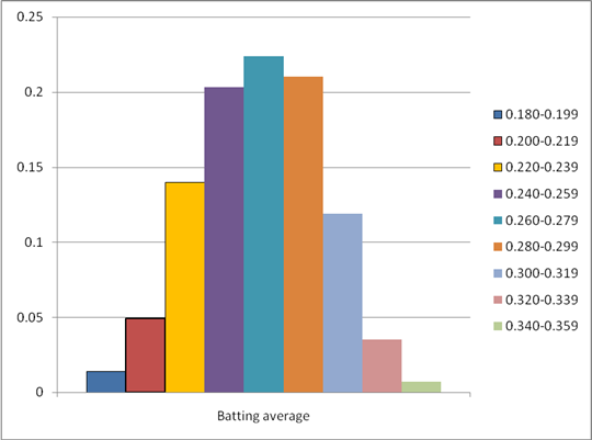
From the above two histograms, we can see that the relative frequency for National league is bit higher than the National League.
Hence, the batting averages tend to be a bit higher in the National League.
Want to see more full solutions like this?
Chapter 2 Solutions
Elementary Statistics ( 3rd International Edition ) Isbn:9781260092561
Additional Math Textbook Solutions
Precalculus: A Unit Circle Approach (3rd Edition)
College Algebra (Collegiate Math)
Intermediate Algebra (13th Edition)
Introductory Statistics
Basic College Mathematics


- Consider the hypothesis test Ho: = 622 against H₁: 6 > 62. Suppose that the sample sizes are n₁ = 20 and n₂ = 8, and that = 4.5; s=2.3. Use a = 0.01. (a) Test the hypothesis. Round your answers to two decimal places (e.g. 98.76). The test statistic is fo = i The critical value is f = Conclusion: i the null hypothesis at a = 0.01. (b) Construct the confidence interval on 02/022 which can be used to test the hypothesis: (Round your answer to two decimal places (e.g. 98.76).) iarrow_forward2011 listing by carmax of the ages and prices of various corollas in a ceratin regionarrow_forwardس 11/ أ . اذا كانت 1 + x) = 2 x 3 + 2 x 2 + x) هي متعددة حدود محسوبة باستخدام طريقة الفروقات المنتهية (finite differences) من جدول البيانات التالي للدالة (f(x . احسب قيمة . ( 2 درجة ) xi k=0 k=1 k=2 k=3 0 3 1 2 2 2 3 αarrow_forward
- 1. Differentiate between discrete and continuous random variables, providing examples for each type. 2. Consider a discrete random variable representing the number of patients visiting a clinic each day. The probabilities for the number of visits are as follows: 0 visits: P(0) = 0.2 1 visit: P(1) = 0.3 2 visits: P(2) = 0.5 Using this information, calculate the expected value (mean) of the number of patient visits per day. Show all your workings clearly. Rubric to follow Definition of Random variables ( clearly and accurately differentiate between discrete and continuous random variables with appropriate examples for each) Identification of discrete random variable (correctly identifies "number of patient visits" as a discrete random variable and explains reasoning clearly.) Calculation of probabilities (uses the probabilities correctly in the calculation, showing all steps clearly and logically) Expected value calculation (calculate the expected value (mean)…arrow_forwardif the b coloumn of a z table disappeared what would be used to determine b column probabilitiesarrow_forwardConstruct a model of population flow between metropolitan and nonmetropolitan areas of a given country, given that their respective populations in 2015 were 263 million and 45 million. The probabilities are given by the following matrix. (from) (to) metro nonmetro 0.99 0.02 metro 0.01 0.98 nonmetro Predict the population distributions of metropolitan and nonmetropolitan areas for the years 2016 through 2020 (in millions, to four decimal places). (Let x, through x5 represent the years 2016 through 2020, respectively.) x₁ = x2 X3 261.27 46.73 11 259.59 48.41 11 257.96 50.04 11 256.39 51.61 11 tarrow_forward
- If the average price of a new one family home is $246,300 with a standard deviation of $15,000 find the minimum and maximum prices of the houses that a contractor will build to satisfy 88% of the market valuearrow_forward21. ANALYSIS OF LAST DIGITS Heights of statistics students were obtained by the author as part of an experiment conducted for class. The last digits of those heights are listed below. Construct a frequency distribution with 10 classes. Based on the distribution, do the heights appear to be reported or actually measured? Does there appear to be a gap in the frequencies and, if so, how might that gap be explained? What do you know about the accuracy of the results? 3 4 555 0 0 0 0 0 0 0 0 0 1 1 23 3 5 5 5 5 5 5 5 5 5 5 5 5 6 6 8 8 8 9arrow_forwardA side view of a recycling bin lid is diagramed below where two panels come together at a right angle. 45 in 24 in Width? — Given this information, how wide is the recycling bin in inches?arrow_forward
- 1 No. 2 3 4 Binomial Prob. X n P Answer 5 6 4 7 8 9 10 12345678 8 3 4 2 2552 10 0.7 0.233 0.3 0.132 7 0.6 0.290 20 0.02 0.053 150 1000 0.15 0.035 8 7 10 0.7 0.383 11 9 3 5 0.3 0.132 12 10 4 7 0.6 0.290 13 Poisson Probability 14 X lambda Answer 18 4 19 20 21 22 23 9 15 16 17 3 1234567829 3 2 0.180 2 1.5 0.251 12 10 0.095 5 3 0.101 7 4 0.060 3 2 0.180 2 1.5 0.251 24 10 12 10 0.095arrow_forwardstep by step on Microssoft on how to put this in excel and the answers please Find binomial probability if: x = 8, n = 10, p = 0.7 x= 3, n=5, p = 0.3 x = 4, n=7, p = 0.6 Quality Control: A factory produces light bulbs with a 2% defect rate. If a random sample of 20 bulbs is tested, what is the probability that exactly 2 bulbs are defective? (hint: p=2% or 0.02; x =2, n=20; use the same logic for the following problems) Marketing Campaign: A marketing company sends out 1,000 promotional emails. The probability of any email being opened is 0.15. What is the probability that exactly 150 emails will be opened? (hint: total emails or n=1000, x =150) Customer Satisfaction: A survey shows that 70% of customers are satisfied with a new product. Out of 10 randomly selected customers, what is the probability that at least 8 are satisfied? (hint: One of the keyword in this question is “at least 8”, it is not “exactly 8”, the correct formula for this should be = 1- (binom.dist(7, 10, 0.7,…arrow_forwardKate, Luke, Mary and Nancy are sharing a cake. The cake had previously been divided into four slices (s1, s2, s3 and s4). What is an example of fair division of the cake S1 S2 S3 S4 Kate $4.00 $6.00 $6.00 $4.00 Luke $5.30 $5.00 $5.25 $5.45 Mary $4.25 $4.50 $3.50 $3.75 Nancy $6.00 $4.00 $4.00 $6.00arrow_forward
 Big Ideas Math A Bridge To Success Algebra 1: Stu...AlgebraISBN:9781680331141Author:HOUGHTON MIFFLIN HARCOURTPublisher:Houghton Mifflin Harcourt
 Holt Mcdougal Larson Pre-algebra: Student Edition...AlgebraISBN:9780547587776Author:HOLT MCDOUGALPublisher:HOLT MCDOUGAL
 Glencoe Algebra 1, Student Edition, 9780079039897...AlgebraISBN:9780079039897Author:CarterPublisher:McGraw Hill