
Concept explainers
Videos
Temperatures are measured at various points on a heatedplate (Table P20.60). Estimate the temperature at (a)
TABLE P20.60 Temperatures
|
|
|
|
|
|
|
|
|
100.00 | 90.00 | 80.00 | 70.00 | 60.00 |
|
|
85.00 | 64.49 | 53.50 | 48.15 | 50.00 |
|
|
70.00 | 48.90 | 38.43 | 35.03 | 40.00 |
|
|
55.00 | 38.78 | 30.39 | 27.07 | 30.00 |
|
|
40.00 | 35.00 | 30.00 | 25.00 | 20.00 |
(a)
To calculate: The value of temperature at
| 100.00 | 90.00 | 80.00 | 70.00 | 60.00 | |
| 85.00 | 64.49 | 53.50 | 48.15 | 50.00 | |
| 70.00 | 48.90 | 38.43 | 35.03 | 40.00 | |
| 55.00 | 38.78 | 30.39 | 27.07 | 30.00 | |
| 40.00 | 35.00 | 30.00 | 25.00 | 20.00 |
Answer to Problem 60P
Solution:
The value of temperature at
Explanation of Solution
Given Information:
The data is provided as,
| 100.00 | 90.00 | 80.00 | 70.00 | 60.00 | |
| 85.00 | 64.49 | 53.50 | 48.15 | 50.00 | |
| 70.00 | 48.90 | 38.43 | 35.03 | 40.00 | |
| 55.00 | 38.78 | 30.39 | 27.07 | 30.00 | |
| 40.00 | 35.00 | 30.00 | 25.00 | 20.00 |
Formula used:
The zero-order Newton’s interpolation formula:
The first-order/linear Newton’s interpolation formula:
The second- order/quadratic Newton’s interpolating polynomial is given by,
Where,
The first finite divided difference is,
And, the n th finite divided difference is,
Calculation:
To calculate the temperature
First use the linear interpolation formula and arrange the points as close to about
The values are,
And,
First calculate
Put in above equation,
Similarly for quadratic interpolation,
Now calculate
Put in quadratic interpolation equation,
Now, do it for cubic interpolation by the use of the formula,
Now calculate
Put in cubic interpolation equation,
And, the error is calculated as,
Similarly the other dividend can be calculated as shown above,
Therefore, the difference table can be summarized for
| Order | Error | |
| 0 | 38.43 | 6.028 |
| 1 | 44.458 | |
| 2 | 43.6144 | |
| 3 | 43.368 | |
| 4 | 43.48045 |
Since the minimum error for order third, therefore, it can be concluded that the value of temperature at
(b)
To calculate: The value of temperature at
| 100.00 | 90.00 | 80.00 | 70.00 | 60.00 | |
| 85.00 | 64.49 | 53.50 | 48.15 | 50.00 | |
| 70.00 | 48.90 | 38.43 | 35.03 | 40.00 | |
| 55.00 | 38.78 | 30.39 | 27.07 | 30.00 | |
| 40.00 | 35.00 | 30.00 | 25.00 | 20.00 |
Answer to Problem 60P
Solution:
The value of temperature at
Explanation of Solution
Given Information:
The data is provided as,
| 100.00 | 90.00 | 80.00 | 70.00 | 60.00 | |
| 85.00 | 64.49 | 53.50 | 48.15 | 50.00 | |
| 70.00 | 48.90 | 38.43 | 35.03 | 40.00 | |
| 55.00 | 38.78 | 30.39 | 27.07 | 30.00 | |
| 40.00 | 35.00 | 30.00 | 25.00 | 20.00 |
Formula used:
The zero-order Newton’s interpolation formula:
The first-order/linear Newton’s interpolation formula:
The second- order/quadratic Newton’s interpolating polynomial is given by,
Where,
The first finite divided difference is,
And, the n th finite divided difference is,
Calculation:
To calculate the temperature
Since, this is a two-dimensional interpolation, therefore one way is to use cubic interpolation along the y direction for specific values of x and then go along the x direction for values of y obtained from the previous analysis.
First use the linear interpolation formula and arrange the points as close to about
The values are,
And,
First calculate
Put in above equation,
Similarly for quadratic interpolation,
Now calculate
Put in quadratic interpolation equation,
Now, do it for cubic interpolation by the use of the formula,
Now calculate
Put in cubic interpolation equation,
And, the error is calculated as,
Similarly the other dividend can be calculated as shown above,
Therefore, the difference table can be summarized for
| Order | Error | |
| 0 | 64.49 | |
| 1 | 59.0335 | |
| 2 | 58.411 | |
| 3 | 58.47032 |
Now, do this for
The values are,
And,
First calculate
Put in above equation,
Similarly for quadratic interpolation,
Now calculate
Put in quadratic interpolation equation,
Now, do it for cubic interpolation by the use of the formula,
Now calculate
Put in cubic interpolation equation,
Similarly, for
Now for the calculation for
The values are,
And,
First calculate
Put in above equation,
Similarly for quadratic interpolation,
Now calculate
Put in quadratic interpolation equation,
Now, do it for cubic interpolation by the use of the formula,
Now calculate
Put in cubic interpolation equation,
And, the error is calculated as,
Similarly the other dividend can be calculated as shown above,
Therefore, the difference table can be summarized for
| Order | Error | |
| 0 | 47.15 | |
| 1 | 46.4885 | |
| 2 | 46.0479875 | |
| 3 | 46.140425 |
Hence, the value of temperature at
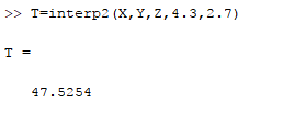
This problem can also be solved with MATLAB as it contains the predefined function interp2.
The MATLAB code is as shown below,
The output in the command window is,
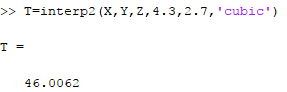
For more accuracy, the result can also be obtained from the bicubic interpolation as shown below,
Finally, the interpolation can also be implemented with the use of splines as shown below,
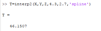
Hence, it can be concluded that the result is similar to that obtained from the calculation.
Want to see more full solutions like this?
Chapter 20 Solutions
Numerical Methods for Engineers


- Complex Analysis 2 First exam Q1: Evaluate f the Figure. 23+3 z(z-i)² 2024-2025 dz, where C is the figure-eight contour shown in C₂arrow_forwardQ/ Find the Laurent series of (2-3) cos around z = 1 2-1arrow_forward31.5. Let be the circle |+1| = 2 traversed twice in the clockwise direction. Evaluate dz (22 + 2)²arrow_forward
- Using FDF, BDF, and CDF, find the first derivative; 1. The distance x of a runner from a fixed point is measured (in meters) at an interval of half a second. The data obtained is: t 0 x 0 0.5 3.65 1.0 1.5 2.0 6.80 9.90 12.15 Use CDF to approximate the runner's velocity at times t = 0.5s and t = 1.5s 2. Using FDF, BDF, and CDF, find the first derivative of f(x)=x Inx for an input of 2 assuming a step size of 1. Calculate using Analytical Solution and Absolute Relative Error: = True Value - Approximate Value| x100 True Value 3. Given the data below where f(x) sin (3x), estimate f(1.5) using Langrage Interpolation. x 1 1.3 1.6 1.9 2.2 f(x) 0.14 -0.69 -0.99 -0.55 0.31 4. The vertical distance covered by a rocket from t=8 to t=30 seconds is given by: 30 x = Loo (2000ln 140000 140000 - 2100 9.8t) dt Using the Trapezoidal Rule, n=2, find the distance covered. 5. Use Simpson's 1/3 and 3/8 Rule to approximate for sin x dx. Compare the results for n=4 and n=8arrow_forward1. A Blue Whale's resting heart rate has period that happens to be approximately equal to 2π. A typical ECG of a whale's heartbeat over one period may be approximated by the function, f(x) = 0.005x4 2 0.005x³-0.364x² + 1.27x on the interval [0, 27]. Find an nth-order Fourier approximation to the Blue Whale's heartbeat, where n ≥ 3 is different from that used in any other posts on this topic, to generate a periodic function that can be used to model its heartbeat, and graph your result. Be sure to include your chosen value of n in your Subject Heading.arrow_forward7. The demand for a product, in dollars, is p = D(x) = 1000 -0.5 -0.0002x² 1 Find the consumer surplus when the sales level is 200. [Hints: Let pm be the market price when xm units of product are sold. Then the consumer surplus can be calculated by foam (D(x) — pm) dx]arrow_forward
- 4. Find the general solution and the definite solution for the following differential equations: (a) +10y=15, y(0) = 0; (b) 2 + 4y = 6, y(0) =arrow_forward5. Find the solution to each of the following by using an appropriate formula developed in the lecture slides: (a) + 3y = 2, y(0) = 4; (b) dy - 7y = 7, y(0) = 7; (c) 3d+6y= 5, y(0) = 0arrow_forward1. Evaluate the following improper integrals: (a) fe-rt dt; (b) fert dt; (c) fi da dxarrow_forward
 College Algebra (MindTap Course List)AlgebraISBN:9781305652231Author:R. David Gustafson, Jeff HughesPublisher:Cengage Learning
 Algebra: Structure And Method, Book 1AlgebraISBN:9780395977224Author:Richard G. Brown, Mary P. Dolciani, Robert H. Sorgenfrey, William L. ColePublisher:McDougal Littell
 Mathematics For Machine TechnologyAdvanced MathISBN:9781337798310Author:Peterson, John.Publisher:Cengage Learning,
 Algebra & Trigonometry with Analytic GeometryAlgebraISBN:9781133382119Author:SwokowskiPublisher:Cengage