Concept explainers
Soft tissue follows an exponential deformation behavior in uniaxial tension while it is in the physiologic or normal range of elongation. This can be expressed as
where
To evaluate
In the following table is stress-strain data for heart chordate tendineae (small tendons used to hold heart valves closed during contraction of the heart muscle; these data are from loading the tissue, while different curves are produced on unloading).
|
|
87.8 | 96.6 | 176 | 263 | 351 | 571 | 834 | 1229 | 1624 | 2107 | 2678 | 3380 | 4258 |
|
|
153 | 204 | 255 | 306 | 357 | 408 | 459 | 510 | 561 | 612 | 663 | 714 | 765 |
Calculate the derivative
Plot the stress versus strain data points along with the analytic curve expressed by the first equation. This will indicate how well the analytic curve matches these data.
Many times this does not work well because the value of
Using this approach, experimental data that are well defined will produce a good match of the data points and the analytic curve. Use this new relationship and again plot the stress versus strain data points and this new analytic curve.
To calculate: The values of
Answer to Problem 16P
Solution: The function that fits the data perfectly is
Explanation of Solution
Given Information:
The provided values of the stress
| 87.8 | 96.6 | 176 | 263 | 351 | 571 | |
| 153 | 204 | 255 | 306 | 357 | 408 |
And,
| 834 | 1229 | 1624 | 2107 | 2678 | 3380 | 4258 | |
| 459 | 510 | 561 | 612 | 663 | 714 | 765 |
Formula Used:
The formula for the derivative of a function at a point c using forward difference is:
The formula for the derivative of a function at a point c using backward difference is:
The formula for the derivative of a function at a point c using central difference is:
Calculation:
Consider the formula for the stress:
Differentiate both sides with respect to
This is a linear equation.
First obtain the value of the derivative of the stress
Now the derivative at the second data point can be obtained using the central difference. Note that the data is equally spaced with a step-size of 51.
Now do the same for all the data points except the last one:
And,
And,
And,
And,
Now the derivative at the last data point can be obtained using the backward difference. Note that the data is equally spaced with a step-size of 51.
Hence, the derivatives have been obtained as:
Now perform a regression analysis on the derivative with respect to
This can be done using MS-Excel.
Step 1: Enter the data points in a blank workbook.
Step 2: Select the data points, go to insert and the select scatter plot.
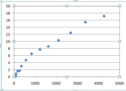
This gives:

It can be seen that the first four points do not follow a linear relationship. So disregard the first four points and obtain a line of best fit for the remaining points.
This can be done using MATLAB.
Code:
Output:

This implies that the linear model for the derivative is:
This gives the value of a as 0.0035499643 and the value of
Now, substitute this in the formula for stress to obtain:
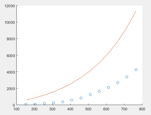
To check whether this model is a good fit for the data, plot this model along with the provided data points. This can be done using MATLAB.
Code:
Output:

Clearly, the obtained function is not a good fit for the data.
Rewrite the expression for the original functionto obtain:
Use this to obtain:
Now consider a data point in the middle of the data
Use this to get the formula for the strain as:
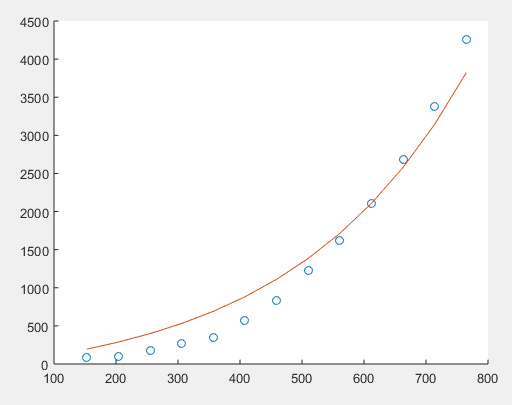
To check whether this model is a good fit for the data, plot this model along with the provided data points. This can be done using MATLAB.
Code:
Output:

It is clear that the function obtained using the data point from the middle is a much better fit for the provided data points.
Hence, the desired function that fits the data points is
Want to see more full solutions like this?
Chapter 20 Solutions
Numerical Methods for Engineers
Additional Math Textbook Solutions
Algebra and Trigonometry (6th Edition)
Calculus: Early Transcendentals (2nd Edition)
Thinking Mathematically (6th Edition)
Elementary Statistics ( 3rd International Edition ) Isbn:9781260092561
A Problem Solving Approach To Mathematics For Elementary School Teachers (13th Edition)
College Algebra (Collegiate Math)
- please help me solvearrow_forwardGolden Ratio search Method f(x) = 2x^3 - 3x^2 - 12x + 1 Golden ratio search rules 1.If f(x) < f(x2): 1. Eliminate all x values less than x2 2. X2 becomes the new a 3. x, becomes the new x2 4. no change in b If f(x) > f(x2): 1. Eliminate all x values greater than x 2. x, becomes the new b 3. x2 becomes the new x 4. no change in aquesion=Narrow the interval in which the minimizer of the function f is located using the golden search method, starting with the initial interval (0,6], until its width is less than 2. Then, accept the midpoint of this interval as an approximate value of the minimizer of the function fand determine it. (ф=0.62)According to the question above, fill in the table below using the algorithm until the appropriate place.please write every step by step in a verry comprehensive wayarrow_forwardIn preparing for the upcoming holiday season, Fresh Toy Company (FTC) designed a new doll called The Dougie that teaches children how to dance. The fixed cost to produce the doll is $100,000. The variable cost, which includes material, labor, and shipping costs, is $31 per doll. During the holiday selling season, FTC will sell the dolls for $39 each. If FTC overproduces the dolls, the excess dolls will be sold in January through a distributor who has agreed to pay FTC $10 per doll. Demand for new toys during the holiday selling season is extremely uncertain. Forecasts are for expected sales of 60,000 dolls with a standard deviation of 15,000. The normal probability distribution is assumed to be a good description of the demand. FTC has tentatively decided to produce 60,000 units (the same as average demand), but it wants to conduct an analysis regarding this production quantity before finalizing the decision. (a) Determine the equation for computing FTC's profit for given values of the…arrow_forward
- For all integers a and b, (a + b)^3 ≡ a^3 + b^3 (mod 3).arrow_forwardLet Χ be a real-valued character (mod k). Let k S = Σnx(n). n=1 If (a, k) = 1, ax(a)S = S (mod k). (iii) Write k = 2ºq where q is odd. Show that there is an integer a with (a, k) = 1 such that a = 3 (mod 2ª) and a = 2 (mod q). Deduce that 12S = 0 (mod k).arrow_forwardProve that (1) Σσς (α) μ(η/α) = n d/n (ii) Σσς(d) = η Σσο(α)/d d❘n d❘n (iii) σ (d) σ (n/d) = Σ d³oo(d) σo(n/d). d|n dnarrow_forward
 Linear Algebra: A Modern IntroductionAlgebraISBN:9781285463247Author:David PoolePublisher:Cengage Learning
