Concept explainers
Dynamic viscosity of water
| T | 0 | 5 | 10 | 20 | 30 | 40 |
|
|
1.787 | 1.519 | 1.307 | 1.002 | 0.7975 | 0.6529 |
(a) Plot these data.
(b) Use interpolation to predict
(c) Use polynomial regression to fit a parabola to these data in order to make the same prediction.
(a)
To graph: The given data if
| T | 0 | 5 | 10 | 20 | 30 | 40 |
| 1.787 | 1.519 | 1.307 | 1.002 | 0.7975 | 0.6529 |
Explanation of Solution
Given Information:
The data is,
| T | 0 | 5 | 10 | 20 | 30 | 40 |
| 1.787 | 1.519 | 1.307 | 1.002 | 0.7975 | 0.6529 |
Graph:
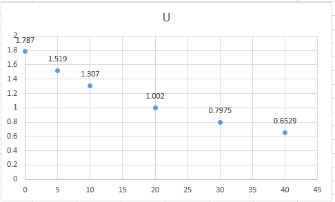
The plot can be easily made with the help of excel as shown below,
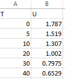
Step 1. First put the data in the excel as shown below,

Step 2. Now click on insert and then scatter plot.
Thus, the scatter plot is,

Interpretation:
From the plot, this can be interpreted that the dynamic viscosity of water decreases as the temperature increases.
(b)
To calculate: The value of
| T | 0 | 5 | 10 | 20 | 30 | 40 |
| 1.787 | 1.519 | 1.307 | 1.002 | 0.7975 | 0.6529 |
Answer to Problem 48P
Solution:
The value of
Explanation of Solution
Given Information:
The data is,
| T | 0 | 5 | 10 | 20 | 30 | 40 |
| 1.787 | 1.519 | 1.307 | 1.002 | 0.7975 | 0.6529 |
Formula used:
The zero-order Newton’s interpolation formula:
The first-order Newton’s interpolation formula:
The second- order Newton’s interpolating polynomial is given by,
The n th-order Newton’s interpolating polynomial is given by,
Where,
The first finite divided difference is,
And, the n th finite divided difference is,
Calculation:
To solve for
Assume
First, order the provided value as close to 7.5 as below,
Therefore,
And,
The first divided difference is,
Thus, the first degree polynomial value can be calculated as,
Put
Solve for other values as,
And,
Similarly,
The second divided difference is,
Thus, the second degree polynomial value can be calculated as,
Put
And,
The third divided difference is,
Thus, the third degree polynomial value can be calculated as,
Put this in above equation,
Therefore,
And, the error is calculated as,
Similarly the other dividend can be calculated as shown above,
Therefore, the difference table can be summarized for
| Order | Error | |
| 0 | ||
| 1 | ||
| 2 | ||
| 3 | ||
| 4 | ||
| 5 |
Since the minimum error for order four, therefore, it can be concluded that the value of
(c)
To calculate: The value of
| T | 0 | 5 | 10 | 20 | 30 | 40 |
| 1.787 | 1.519 | 1.307 | 1.002 | 0.7975 | 0.6529 |
Answer to Problem 48P
Solution:
The value of
Explanation of Solution
Given Information:
The data is,
| T | 0 | 5 | 10 | 20 | 30 | 40 |
| 1.787 | 1.519 | 1.307 | 1.002 | 0.7975 | 0.6529 |
Calculation:
This problem can be easily solved with the help of excel as shown below,
Step 1. First put the data in the excel as shown below,

Step 2. Now click on insert and then scatter plot.
Step 3. Click on layout, Trendline, more trendline options, polynomial and then display equation on chart.
Step 4. Click on display R-squared value on chart as shown below,

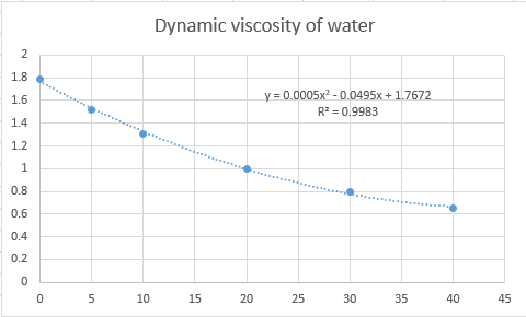
Thus, the final plot is shown as below,

Therefore, the regression plot equation of the data will be,
Put
Hence, the value of
Want to see more full solutions like this?
Chapter 20 Solutions
Numerical Methods for Engineers
- 1. Evaluate the following improper integrals: (a) fe-rt dt; (b) fert dt; (c) fi da dxarrow_forward8. Given the rate of net investment I(t) = 9t¹/2, find the level of capital formation in (i) 16 years and (ii) between the 4th and the 8th years.arrow_forward9. If the marginal revenue function of a firm in the production of output is MR = 40 - 10q² where q is the level of output, and total revenue is 120 at 3 units of output, find the total revenue function. [Hints: TR = √ MRdq]arrow_forward
- 6. Solve the following first-order linear differential equations; if an initial condition is given, definitize the arbitrary constant: (a) 2 + 12y + 2et = 0, y(0) = /; (b) dy+y=tarrow_forward4. Let A = {a, b, c, d, e, f}, B = {e, f, g, h} and C = {a, e, h,i}. Let U = {a, b, c, d, e, f, g, h, i, j, k}. • Draw a Venn Diagram to describe the relationships between these sets Find (AB) NC • Find (AC) UB Find AUBUC • Find (BC) N (A - C)arrow_forward7. A consumer lives on an island where she produces two goods x and y according to the production possibility frontier x² + y² < 200 and she consumes all the goods. Her utility function is U(x, y) = x y³. She faces an environmental constraint on her total output of both goods. The environmental constraint is given by x + y ≤20. • (a) Write down the consumer's optimization problem. (b) Write out the Kuhn-Tucker first order conditions. (c) Find the consumer's optimal consumption bundle (x*, y*).arrow_forward
- 3. Answer the following questions: (a) Given the marginal propensity to import M'(Y) = 0.1 and the information that M = 20 when Y = 0, find the import function M(Y). (b) Given a continuous income stream at the constant rate of $1,000 per year, what will be the present value II if the income stream terminates after exactly 3 years and the discount rate is 0.04? (c) What is the present value of a perpetual cash flow of $2,460 per year, discounted at r = 8%?arrow_forward5. Let A and B be arbitrary sets. Prove AnB = AUB.arrow_forward2. Answer the following questions: (a) Given the marginal-revenue function R'(Q) = 28Q - €0.3Q, find the total-revenue function R(Q). What initial condition can you introduce to definitize the constant of integration? = (b) Given the marginal propensity to consume C'(Y) 0.80.1Y-1/2 and the information that C = Y when Y = 100, find the consumption function C(Y).arrow_forward
- 7. Let X, A, and B be arbitrary sets such that ACX and BC X. Prove AUB CX.arrow_forward1. Write out the following sets as a list of elements. If necessary you may use ... in your description. {x EZ: |x|< 10 A x < 0} {x ЄN: x ≤ 20 A x = 2y for some y = N} {n EN: 3 | n^ 1 < n < 20} {y Є Z: y² <0}arrow_forward3. For each statement below, write an equivalent statement using the justification given. = y Є A or yЄ B by the definition of union = y Є A or y Є B by the definition of set complement = x = C and x & D by DeMorgan's Law =Vx (x EnFxЄEUF) by definition of subset. = (X CYUZ)A (YUZ CX) by definition of set equalityarrow_forward
- Algebra & Trigonometry with Analytic GeometryAlgebraISBN:9781133382119Author:SwokowskiPublisher:Cengage
 Algebra and Trigonometry (MindTap Course List)AlgebraISBN:9781305071742Author:James Stewart, Lothar Redlin, Saleem WatsonPublisher:Cengage Learning
 Functions and Change: A Modeling Approach to Coll...AlgebraISBN:9781337111348Author:Bruce Crauder, Benny Evans, Alan NoellPublisher:Cengage Learning
 College AlgebraAlgebraISBN:9781305115545Author:James Stewart, Lothar Redlin, Saleem WatsonPublisher:Cengage Learning


