
Videos
Human blood behaves as a Newtonian fluid (see Prob. 20.55) in the high shear rate region where
where
|
|
0.91 | 3.3 | 4.1 | 6.3 | 9.6 | 23 | 36 | 49 | 65 | 105 | 126 | 215 | 315 | 402 |
|
|
0.059 | 0.15 | 0.19 | 0.27 | 0.39 | 0.87 | 1.33 | 1.65 | 2.11 | 3.44 | 4.12 | 7.02 | 10.21 | 13.01 |
| Region | Casson | Transition | Newtonian |
Find the values of
To calculate: The values of
| 0.91 | 3.3 | 4.1 | 6.3 | 9.6 | 23 | 36 | 49 | 65 | 105 | 126 | 215 | 315 | 402 | |
| 0.0059 | 0.15 | 0.19 | 0.27 | 0.39 | 0.84 | 1.33 | 1.65 | 2.11 | 3.44 | 4.12 | 7.02 | 10.21 | 13.01 | |
| Region | Casson | Transition | Newtonian | |||||||||||
Also, find the correlation coefficient for each regression analysis. Plot the two regression lines on the Casson plot (
) and extend the regressions lines as dashed lines into adjoining regressions and include the given data points in the plots.
Answer to Problem 15P
Solution: In the Casson region
and in Newtonian region
and in Newtonian region
Explanation of Solution
Given Information: Consider the experimentally measured values of
| 0.91 | 3.3 | 4.1 | 6.3 | 9.6 | 23 | 36 | 49 | 65 | 105 | 126 | 215 | 315 | 402 | |
| 0.0059 | 0.15 | 0.19 | 0.27 | 0.39 | 0.84 | 1.33 | 1.65 | 2.11 | 3.44 | 4.12 | 7.02 | 10.21 | 13.01 | |
| Region | Casson | Transition | Newtonian | |||||||||||
The Casson relationship is with
The relationship for the Newtonian fluid,
Formula used:
If
data points
Here,
If
data points
The correlation coefficient is,
Here,
Calculation:
Consider the experimentally measured values of
| 0.91 | 3.3 | 4.1 | 6.3 | 9.6 | 23 | 36 | 49 | 65 | 105 | 126 | 215 | 315 | 402 | |
| 0.0059 | 0.15 | 0.19 | 0.27 | 0.39 | 0.84 | 1.33 | 1.65 | 2.11 | 3.44 | 4.12 | 7.02 | 10.21 | 13.01 | |
| Region | Casson | Transition | Newtonian | |||||||||||
The Casson relationship is with
Defining the two variables
Therefore, the unknown constant
Construct the following table considering the data in the Casson regions to compute the unknown constant
| 1 | 0.91 | 0.0059 | 0.95394 | 0.07681 | 0.91000 | 0.07327 |
| 2 | 3.3 | 0.15 | 1.81659 | 0.38730 | 3.30000 | 0.70356 |
| 3 | 4.1 | 0.19 | 2.02485 | 0.43589 | 4.10000 | 0.88261 |
| 4 | 6.3 | 0.27 | 2.50998 | 0.51962 | 6.30000 | 1.30422 |
| 5 | 9.6 | 0.39 | 3.09839 | 0.62450 | 9.60000 | 1.93494 |
| 6 | 23 | 0.84 | 4.79583 | 0.91652 | 23.00000 | 4.39545 |
| 7 | 36 | 1.33 | 6.00000 | 1.15326 | 36.00000 | 6.91954 |
| 21.19957 | 4.11389 | 83.21000 | 16.21360 |
Therefore, the unknown constant
Therefore,
Hence, the linear regression line for Casson region is,
Construct the table to calculate the correlation coefficients defining
| 1 | 0.95394 | 0.07681 | 0.26101 | 0.17789 | 0.01022 |
| 2 | 1.81659 | 0.38730 | 0.04016 | 0.34830 | 0.00152 |
| 3 | 2.02485 | 0.43589 | 0.02305 | 0.38944 | 0.00216 |
| 4 | 2.50998 | 0.51962 | 0.00463 | 0.48527 | 0.00118 |
| 5 | 3.09839 | 0.62450 | 0.00135 | 0.60151 | 0.00053 |
| 6 | 4.79583 | 0.91652 | 0.10812 | 0.93682 | 0.00041 |
| 7 | 6.00000 | 1.15326 | 0.31986 | 1.17469 | 0.00046 |
| 0.75818 | 0.01648 |
Therefore,
Hence, the correlation coefficients,
Therefore, for Casson region the linear fit is,
And the correlation coefficients,
Consider the Newtonian relationship as,
From the linear regression,
Construct the following table considering the data in the Newton regions to compute the unknown constant
| 1 | 105 | 3.44 | 11025 | 361.20 |
| 2 | 126 | 4.12 | 15876 | 519.12 |
| 3 | 215 | 7.02 | 46225 | 1509.30 |
| 4 | 315 | 10.21 | 99225 | 3216.15 |
| 5 | 402 | 13.01 | 161604 | 5230.02 |
| 37.8 | 333955 | 10835.79 |
Therefore, the unknown constant
Therefore,
Hence, the linear regression line for Newtonian region is,
Construct the table to calculate the correlation coefficients defining
| 1 | 105 | 3.44 | 16.97440 | 3.40725 | 0.00107 |
| 2 | 126 | 4.12 | 16.97440 | 4.08870 | 0.00098 |
| 3 | 215 | 7.02 | 49.28040 | 6.97675 | 0.00187 |
| 4 | 315 | 10.21 | 104.24410 | 10.22175 | 0.00014 |
| 5 | 402 | 13.01 | 169.26010 | 13.04490 | 0.00122 |
| 356.73340 | 0.00528 |
Therefore,
Hence, the correlation coefficients,
Therefore, for Newtonian region the linear fit is
And the correlation coefficients,
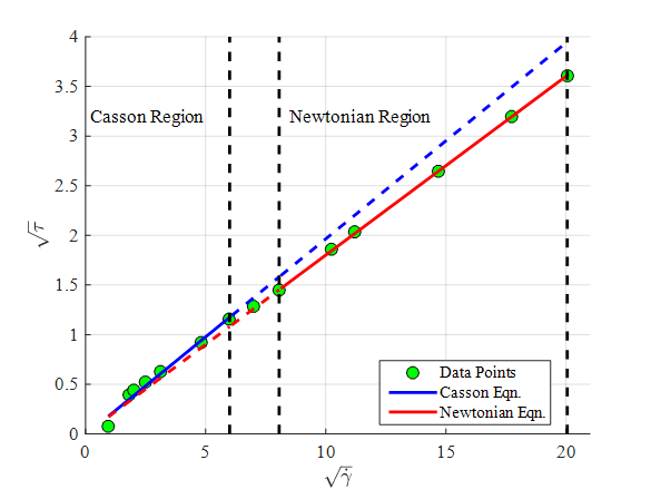
Graph:
Consider the two regression lines in the field of
In the Casson region,
In the Newtonian region,
Construct the MATLAB function ‘Code_97924_20_15a.m’ to plot the two regression lines on the Casson plot (
) and extend the regressions lines as dashed lines into adjoining regressions and include the given data points in the plots.
The comparison is shown on the plot as,
Want to see more full solutions like this?
Chapter 20 Solutions
Numerical Methods for Engineers


- Can you provide steps and an explaination on how the height value to calculate the Pressure at point B is (-5-3.5) and the solution is 86.4kPa.arrow_forwardPROBLEM 3.46 The solid cylindrical rod BC of length L = 600 mm is attached to the rigid lever AB of length a = 380 mm and to the support at C. When a 500 N force P is applied at A, design specifications require that the displacement of A not exceed 25 mm when a 500 N force P is applied at A For the material indicated determine the required diameter of the rod. Aluminium: Tall = 65 MPa, G = 27 GPa. Aarrow_forwardFind the equivalent mass of the rocker arm assembly with respect to the x coordinate. k₁ mi m2 k₁arrow_forward
- 2. Figure below shows a U-tube manometer open at both ends and containing a column of liquid mercury of length l and specific weight y. Considering a small displacement x of the manometer meniscus from its equilibrium position (or datum), determine the equivalent spring constant associated with the restoring force. Datum Area, Aarrow_forward1. The consequences of a head-on collision of two automobiles can be studied by considering the impact of the automobile on a barrier, as shown in figure below. Construct a mathematical model (i.e., draw the diagram) by considering the masses of the automobile body, engine, transmission, and suspension and the elasticity of the bumpers, radiator, sheet metal body, driveline, and engine mounts.arrow_forward3.) 15.40 – Collar B moves up at constant velocity vB = 1.5 m/s. Rod AB has length = 1.2 m. The incline is at angle = 25°. Compute an expression for the angular velocity of rod AB, ė and the velocity of end A of the rod (✓✓) as a function of v₂,1,0,0. Then compute numerical answers for ȧ & y_ with 0 = 50°.arrow_forward
- 2.) 15.12 The assembly shown consists of the straight rod ABC which passes through and is welded to the grectangular plate DEFH. The assembly rotates about the axis AC with a constant angular velocity of 9 rad/s. Knowing that the motion when viewed from C is counterclockwise, determine the velocity and acceleration of corner F.arrow_forward500 Q3: The attachment shown in Fig.3 is made of 1040 HR. The static force is 30 kN. Specify the weldment (give the pattern, electrode number, type of weld, length of weld, and leg size). Fig. 3 All dimension in mm 30 kN 100 (10 Marks)arrow_forward(read image) (answer given)arrow_forward
- A cylinder and a disk are used as pulleys, as shown in the figure. Using the data given in the figure, if a body of mass m = 3 kg is released from rest after falling a height h 1.5 m, find: a) The velocity of the body. b) The angular velocity of the disk. c) The number of revolutions the cylinder has made. T₁ F Rd = 0.2 m md = 2 kg T T₂1 Rc = 0.4 m mc = 5 kg ☐ m = 3 kgarrow_forward(read image) (answer given)arrow_forward11-5. Compute all the dimensional changes for the steel bar when subjected to the loads shown. The proportional limit of the steel is 230 MPa. 265 kN 100 mm 600 kN 25 mm thickness X Z 600 kN 450 mm E=207×103 MPa; μ= 0.25 265 kNarrow_forward
 Principles of Heat Transfer (Activate Learning wi...Mechanical EngineeringISBN:9781305387102Author:Kreith, Frank; Manglik, Raj M.Publisher:Cengage Learning