
Videos
SAT Scores. The SAT is a standardized test used by many colleges and universities in their admission decisions. More than one million high school students take the SAT each year. The current version of the SAT includes three parts: reading comprehension, mathematics, and writing. A perfect combined score for all three parts is 2400. A sample of SAT scores for the combined three-part SAT are as follows:
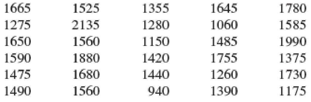
- a. Show a frequency distribution and histogram. Begin with the first class starting at 800 and use a class width of 200.
- b. Comment on the shape of the distribution.
- c. What other observations can be made about the SAT scores based on the tabular and graphical summaries?
a.
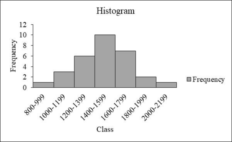
Construct the frequency distribution and histogram for the data.
Answer to Problem 44SE
The frequency distribution is tabulated below:
| Class | Tally | Frequency |
| 800-999 | 1 | |
| 1000-1199 | 3 | |
| 1200-1399 | 6 | |
| 1400-1599 | 10 | |
| 1600-1799 | 7 | |
| 1800-1999 | 2 | |
| 2000-2199 | 1 | |
| Total | 30 |
- Output using EXCEL is given below:
Explanation of Solution
Calculation:
The data represent the sample of SAT scores for the combined three part sat scores.
The frequencies are calculated using the tally mark and the method of grouping is also used because the range of the data is from 800 to 2,199. Here, the number of times each class level repeats is the frequency of that particular class.
- From the given data set, it is given that the class should be approximately started from 800 with the class width of 200.
- Make a tally mark for each value in the corresponding class and continue for all the values in the data.
- The number of tally marks in each class represents the frequency f of that class.
Similarly, the frequency of the remaining classes for the data set is given below:
| Class | Tally | Frequency |
| 800-999 | 1 | |
| 1000-1199 | 3 | |
| 1200-1399 | 6 | |
| 1400-1599 | 10 | |
| 1600-1799 | 7 | |
| 1800-1999 | 2 | |
| 2000-2199 | 1 | |
| Total | 30 |
Software procedure:
Step-by-step procedure to draw the frequency histogram chart using EXCEL software:
- In Excel sheet, enter Class in one column and Frequency in another column.
- Select the data and then choose Insert > Insert Column Bar Charts.
- Select Clustered Column Under More Column Charts.
- Double click the bars
- In Format Data Series, enter 0 in Gap Width under Series Options.
b.
Comment the shape of the distribution.
Answer to Problem 44SE
The distribution of sat score is approximately symmetric.
Explanation of Solution
Symmetric distribution:
When the left and right sides of the distribution are approximately equal or mirror images of each other, then the distribution is called as a symmetric distribution. A symmetric distribution can be U shaped or bell shaped.
From the graph, it is observed that the left and right sides of the histogram are approximately equal. In addition, the shape of the distribution is a bell-shaped curve.
Thus, it can be concluded that the distribution is approximately symmetric.
c.
Comment the observations of sat scores based on the tabular and graphical summary.
Explanation of Solution
- From the data and the histogram, it is observed that approximately 33 percent of sat score (frequency about 10 of 30) lie between 1,400 and 1,599, which is modal class of the distribution. The average value of sat scores is 1,500.
- Moreover, the scores, which are less than 800 or greater than 2,200, are unusual.
Want to see more full solutions like this?
Chapter 2 Solutions
Essentials of Statistics for Business and Economics


- You find out that the dietary scale you use each day is off by a factor of 2 ounces (over — at least that’s what you say!). The margin of error for your scale was plus or minus 0.5 ounces before you found this out. What’s the margin of error now?arrow_forwardSuppose that Sue and Bill each make a confidence interval out of the same data set, but Sue wants a confidence level of 80 percent compared to Bill’s 90 percent. How do their margins of error compare?arrow_forwardSuppose that you conduct a study twice, and the second time you use four times as many people as you did the first time. How does the change affect your margin of error? (Assume the other components remain constant.)arrow_forward
- Out of a sample of 200 babysitters, 70 percent are girls, and 30 percent are guys. What’s the margin of error for the percentage of female babysitters? Assume 95 percent confidence.What’s the margin of error for the percentage of male babysitters? Assume 95 percent confidence.arrow_forwardYou sample 100 fish in Pond A at the fish hatchery and find that they average 5.5 inches with a standard deviation of 1 inch. Your sample of 100 fish from Pond B has the same mean, but the standard deviation is 2 inches. How do the margins of error compare? (Assume the confidence levels are the same.)arrow_forwardA survey of 1,000 dental patients produces 450 people who floss their teeth adequately. What’s the margin of error for this result? Assume 90 percent confidence.arrow_forward
- The annual aggregate claim amount of an insurer follows a compound Poisson distribution with parameter 1,000. Individual claim amounts follow a Gamma distribution with shape parameter a = 750 and rate parameter λ = 0.25. 1. Generate 20,000 simulated aggregate claim values for the insurer, using a random number generator seed of 955.Display the first five simulated claim values in your answer script using the R function head(). 2. Plot the empirical density function of the simulated aggregate claim values from Question 1, setting the x-axis range from 2,600,000 to 3,300,000 and the y-axis range from 0 to 0.0000045. 3. Suggest a suitable distribution, including its parameters, that approximates the simulated aggregate claim values from Question 1. 4. Generate 20,000 values from your suggested distribution in Question 3 using a random number generator seed of 955. Use the R function head() to display the first five generated values in your answer script. 5. Plot the empirical density…arrow_forwardFind binomial probability if: x = 8, n = 10, p = 0.7 x= 3, n=5, p = 0.3 x = 4, n=7, p = 0.6 Quality Control: A factory produces light bulbs with a 2% defect rate. If a random sample of 20 bulbs is tested, what is the probability that exactly 2 bulbs are defective? (hint: p=2% or 0.02; x =2, n=20; use the same logic for the following problems) Marketing Campaign: A marketing company sends out 1,000 promotional emails. The probability of any email being opened is 0.15. What is the probability that exactly 150 emails will be opened? (hint: total emails or n=1000, x =150) Customer Satisfaction: A survey shows that 70% of customers are satisfied with a new product. Out of 10 randomly selected customers, what is the probability that at least 8 are satisfied? (hint: One of the keyword in this question is “at least 8”, it is not “exactly 8”, the correct formula for this should be = 1- (binom.dist(7, 10, 0.7, TRUE)). The part in the princess will give you the probability of seven and less than…arrow_forwardplease answer these questionsarrow_forward
- Selon une économiste d’une société financière, les dépenses moyennes pour « meubles et appareils de maison » ont été moins importantes pour les ménages de la région de Montréal, que celles de la région de Québec. Un échantillon aléatoire de 14 ménages pour la région de Montréal et de 16 ménages pour la région Québec est tiré et donne les données suivantes, en ce qui a trait aux dépenses pour ce secteur d’activité économique. On suppose que les données de chaque population sont distribuées selon une loi normale. Nous sommes intéressé à connaitre si les variances des populations sont égales.a) Faites le test d’hypothèse sur deux variances approprié au seuil de signification de 1 %. Inclure les informations suivantes : i. Hypothèse / Identification des populationsii. Valeur(s) critique(s) de Fiii. Règle de décisioniv. Valeur du rapport Fv. Décision et conclusion b) A partir des résultats obtenus en a), est-ce que l’hypothèse d’égalité des variances pour cette…arrow_forwardAccording to an economist from a financial company, the average expenditures on "furniture and household appliances" have been lower for households in the Montreal area than those in the Quebec region. A random sample of 14 households from the Montreal region and 16 households from the Quebec region was taken, providing the following data regarding expenditures in this economic sector. It is assumed that the data from each population are distributed normally. We are interested in knowing if the variances of the populations are equal. a) Perform the appropriate hypothesis test on two variances at a significance level of 1%. Include the following information: i. Hypothesis / Identification of populations ii. Critical F-value(s) iii. Decision rule iv. F-ratio value v. Decision and conclusion b) Based on the results obtained in a), is the hypothesis of equal variances for this socio-economic characteristic measured in these two populations upheld? c) Based on the results obtained in a),…arrow_forwardA major company in the Montreal area, offering a range of engineering services from project preparation to construction execution, and industrial project management, wants to ensure that the individuals who are responsible for project cost estimation and bid preparation demonstrate a certain uniformity in their estimates. The head of civil engineering and municipal services decided to structure an experimental plan to detect if there could be significant differences in project evaluation. Seven projects were selected, each of which had to be evaluated by each of the two estimators, with the order of the projects submitted being random. The obtained estimates are presented in the table below. a) Complete the table above by calculating: i. The differences (A-B) ii. The sum of the differences iii. The mean of the differences iv. The standard deviation of the differences b) What is the value of the t-statistic? c) What is the critical t-value for this test at a significance level of 1%?…arrow_forward
 Holt Mcdougal Larson Pre-algebra: Student Edition...AlgebraISBN:9780547587776Author:HOLT MCDOUGALPublisher:HOLT MCDOUGAL
 Glencoe Algebra 1, Student Edition, 9780079039897...AlgebraISBN:9780079039897Author:CarterPublisher:McGraw Hill
 Big Ideas Math A Bridge To Success Algebra 1: Stu...AlgebraISBN:9781680331141Author:HOUGHTON MIFFLIN HARCOURTPublisher:Houghton Mifflin Harcourt
 College Algebra (MindTap Course List)AlgebraISBN:9781305652231Author:R. David Gustafson, Jeff HughesPublisher:Cengage Learning